
Regression
Fits x, y pairs by least squares on seven linearised models and picks the best by the typical error in y, after eliminating models with a residual pattern or a term that is not significant.
What it is for
Regression fits a relationship between two measured quantities when you do not know its form in advance: rainfall against runoff, stage against discharge at a gauge, watershed area against peak flow, infiltration rate against time. It answers: which equation describes these data best, and how far off will it typically be?
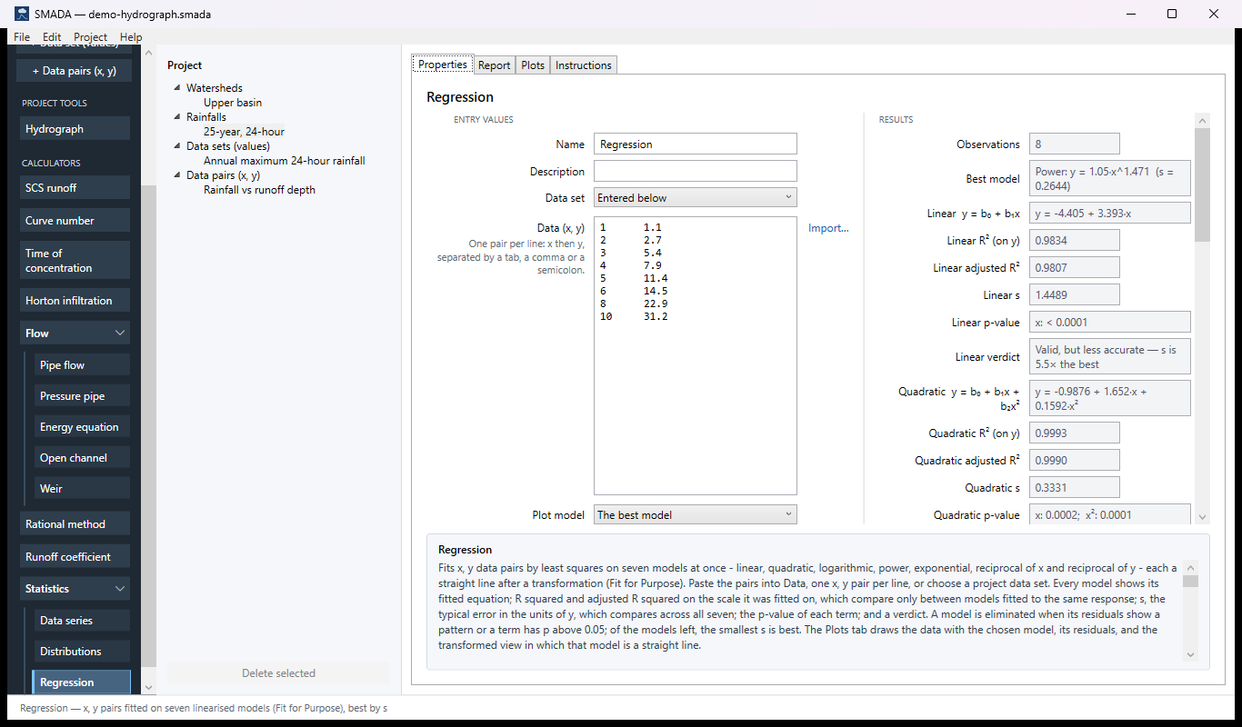
You enter the observations as x, y pairs, one pair per line (two spreadsheet columns paste directly), or choose in Data set a project data set added with the + Data pairs (x, y) button. SMADA fits seven models at once: linear, quadratic, logarithmic, power, exponential, reciprocal of x and reciprocal of y. Each is a straight line after a transformation (the quadratic is a multiple regression on x and x²), fitted by least squares and turned back into y.
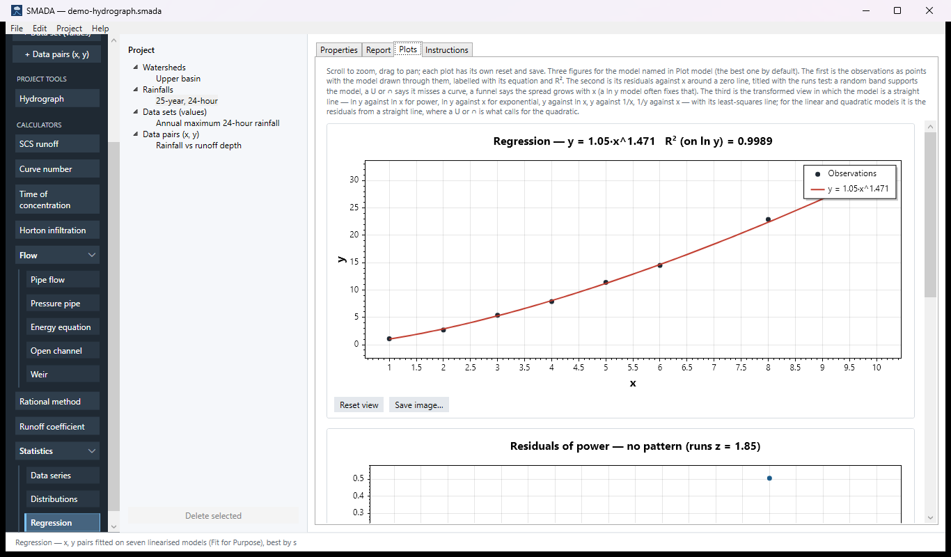
For every model you get the fitted equation, R² and adjusted R² on the scale it was fitted on, s (the typical error in the units of y), the p-value of each term, and a verdict. Following Ron Eaglin's Fit for Purpose method, a model is eliminated when its residuals show a pattern or one of its terms is not significant; of the models left, the one with the smallest s is best. The Plots tab draws the chosen model through the data, its residuals, and the transformed view in which it should be a straight line.
The Regression tabs
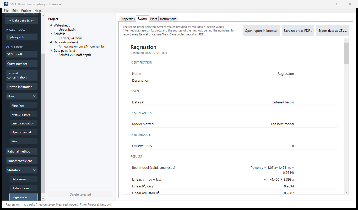
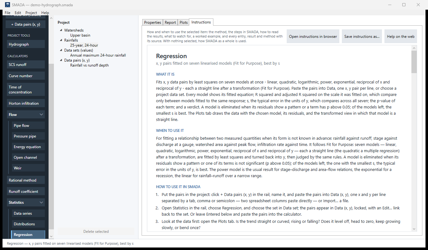
Every item in SMADA has the same four tabs. These are captured from the program with the example values it opens with; select a picture to see it full size.
Properties tab — where you enter values and read the results
Report tab — the same values as a report, ready for HTML, PDF or CSV
Plots tab — what it draws
Instructions tab — the manual page in the program
How it calculates
Each model is made into a linear least-squares problem by transforming x, y or both, fitted, then converted back into y so that every model's error can be measured in the same units. The steps below run for all seven models on every recalculation.
The pairs come from Data (x, y). If a project data set is chosen in Data set, its pairs are copied in and locked; only then does that copy step run. The report names the data set, or says Entered below when the pairs were typed in.
1. The seven models and their transforms
| Model | Equation | Fitted as | Coefficients p | Requirement |
|---|---|---|---|---|
| Linear | y = b0 + b1x | y on x | 2 | none |
| Quadratic | y = b0 + b1x + b2x2 | y on x and x2 | 3 | none |
| Logarithmic | y = b0 + b1 ln x | y on ln x | 2 | every x > 0 |
| Power | y = a xb | ln y on ln x | 2 | every x > 0; every y of one sign |
| Exponential | y = a ebx | ln y on x | 2 | every y of one sign |
| Reciprocal of x | y = b0 + b1/x | y on 1/x | 2 | every x ≠ 0 |
| Reciprocal of y | y = 1 / (b0 + b1x) | 1/y on x | 2 | every y ≠ 0 |
For power and exponential, b0 is fitted as ln a, so a = eb0 and b = b1. When every y is negative they are fitted to −y and a is reported negative. Logarithms are natural logarithms.
A model is fitted to every point or not at all, so that every s is computed over the same data. A model is not fitted, with the reason named, when:
- there are fewer than p + 1 points (3 for the two-coefficient models, 4 for the quadratic);
- the data break the model's requirement in the table;
- a value is not a number, or the transformed x has no spread;
- for the reciprocal of y, the fitted 1/y changes sign relative to y over the data, so it cannot be turned back into y.
2. Least squares on the transformed scale
Each model is an ordinary least-squares fit with an intercept, v = b0 + Σ bj uj, where v is the transformed response (y, ln y or 1/y) and uj are the model's terms (x; x and x2; ln x; 1/x). For numerical stability each term column is first centred and scaled by its mean and population standard deviation, the normal equations are solved by Gauss-Jordan inversion with partial pivoting, and the coefficients are converted back to the original terms:
bj = gj / dj
b0 = g0 − Σ gj ūj / dj
- gj
- coefficient on the centred and scaled term j (g0 the intercept)
- ūj, dj
- mean and population standard deviation of term j over the data
- bj
- coefficient on the original term j, as reported
Centring and scaling do not change the fitted line; they only keep the arithmetic accurate.
3. R² and adjusted R², on the fitted scale
R2 = 1 − SSEv / SSTv
Radj2 = 1 − (1 − R2)(n − 1) / (n − p)
- SSEv
- sum of squared residuals of the transformed response v about the fitted line
- SSTv
- sum of squared deviations of v about its mean
- n
- number of pairs
- p
- number of coefficients, intercept included (2, or 3 for the quadratic)
R² is kept between 0 and 1, and is 1 if v has no spread. Because both are computed on the scale the model was fitted on (y, ln y or 1/y), they compare only between models fitted to the same response, never a ln y fit with a y fit.
4. s, in the units of y
Each model is turned back into y (ŷ = ev̂ for power and exponential, ŷ = 1/v̂ for the reciprocal of y, with the sign restored for negated data), and its residuals are taken in y:
s = √( Σ (yi − ŷi)2 / (n − p) )
- s
- standard error of the model, the typical error, in the units of y
- ŷi
- the model's value at xi, in y units
Every model's s is on the same scale, so s is the number that compares across all seven.
5. Term p-values
Each non-intercept term is tested with a two-sided Student t-test on the least-squares fit (on the fitted scale):
tj = gj / √( MSE · Cjj ), MSE = SSEv / (n − p)
Pj = 2 [ 1 − Ft( |tj|; n − p ) ]
- Cjj
- diagonal element of the inverse of the (scaled) normal-equations matrix
- Ft
- Student t cumulative distribution with n − p degrees of freedom, computed through the regularised incomplete beta function (continued fraction, Numerical Recipes §6.4)
- Pj
- p-value of term j; shown as < 0.0001 when smaller
Scaling a column does not change its t statistic, so this is the usual t-test on bj. An exact fit (standard error zero) gives p = 0. A term with p > 0.05 is not significant.
6. Residual pattern: the runs test
The residuals in y are put in order of x, and their signs are read as runs (stretches of one sign). Residuals no larger than 10−9 times the largest |y| count as zero and are dropped, so an exact fit shows no pattern. The Wald-Wolfowitz statistic is:
E[R] = 1 + 2 n1 n2 / N
Var[R] = 2 n1 n2 (2 n1 n2 − N) / ( N2 (N − 1) )
z = (R − E[R]) / √Var[R]
- R
- number of runs of one sign
- n1, n2
- number of positive and negative residuals
- N
- n1 + n2, the number of non-zero residuals
- z
- runs-test statistic; a large negative z means too few runs
All residuals of one sign give z = −9, as in Fit for Purpose. The model has a residual pattern (it misses a curve) when z < −2 and there are at least 8 points; with fewer than 8 the test is not applied and the verdict says to check the residual plot.
7. Verdicts and the best model
- A fitted model is valid when it has no residual pattern and every term has p ≤ 0.05.
- The best model is the valid one with the smallest s. If no model is valid, the model with the smallest s of all is named, with the reasons it was eliminated.
- Every other valid model with s ≤ 1.3 × the best s is Good.
- A valid model with a larger s is Valid, but less accurate, with its s as a multiple of the best.
- A model with a pattern or a non-significant term is Eliminated, with each reason and the runs z or p-value.
- A model the data cannot take is Not fitted, with the requirement it fails.
Best model shows the winning equation and its s.
What changed from the earlier regression
SMADA's earlier six-form regression fitted each form to whichever points its transform could take, reported r² and a standard error, and named the smallest standard error best. In version 1.1 it was rebuilt on Fit for Purpose: the quadratic was added, a model is fitted to every point or none, adjusted R², term p-values and the runs test were added, and the best model is chosen only from those that pass both checks.
Checking the example by hand
The calculator opens with eight pairs, made to lie close to y proportional to x1.5. The table gives the logarithms too, for checking the power model.
| x | y | ln x | ln y |
|---|---|---|---|
| 1 | 1.1 | 0.0000 | 0.0953 |
| 2 | 2.7 | 0.6931 | 0.9933 |
| 3 | 5.4 | 1.0986 | 1.6864 |
| 4 | 7.9 | 1.3863 | 2.0669 |
| 5 | 11.4 | 1.6094 | 2.4336 |
| 6 | 14.5 | 1.7918 | 2.6741 |
| 8 | 22.9 | 2.0794 | 3.1311 |
| 10 | 31.2 | 2.3026 | 3.4404 |
- Linear: least squares of y on x gives b0 = −4.405 and b1 = 3.393, with R2 = 0.9834 and s = 1.4489 (n − p = 6).
- Power: least squares of ln y on ln x gives b0 = 0.04908 and b1 = 1.4714, so a = e0.04908 = 1.050 and y = 1.050 x1.471. R2 on ln y = 0.9989 and adjusted R2 = 0.9987. Turning each fitted value back into y and summing the squared residuals in y gives s = √(SSE / 6) = 0.2644.
- Power is the best model: it is valid (the runs test gives z = 1.85, no pattern, and its term has p < 0.0001) and has the smallest s. The linear s is 1.4489 / 0.2644 = 5.5 times the best, so the line is valid but less accurate. The quadratic is good, with s = 0.3331, within 1.3 times the best (0.3331 / 0.2644 = 1.26).
The coefficients, R², adjusted R², p-values and runs z of every model were also checked against statsmodels, and the verdicts against an independent implementation of the rules above; all agree.
Sources
- Eaglin, R., Fit for Purpose: Ron Eaglin's method for choosing a regression model (transformations, residual patterns, term significance and s), from his EGN3443 statistics course.
- Wanielista, Kersten and Eaglin, Hydrology: Water Quantity and Quality Control, 2nd ed., Wiley, 1997.
- Wald, A. and Wolfowitz, J., 'On a test whether two samples are from the same population', Ann. Math. Stat. 11, 1940 (runs test).
All SMADA calculators · Get SMADA free for Windows from the Microsoft Store