
Distributions
Fits a record of extremes to seven frequency distributions, compares how well each fits, and gives the chosen one's 2- to 200-year estimates with their standard errors.
What it is for
Distributions is frequency analysis proper. Given a record of extremes, such as annual maximum rainfalls, peak discharges or stages, it answers: which probability distribution describes this record, and what is the 25-, 100- or 500-year value, with how much uncertainty? It is the DISTRIB program (Eaglin and Wanielista) brought into SMADA.
You enter the record, one value per line, typed into Series or taken from a project data set chosen in Data set. You choose a Plotting position formula (Weibull by default), the number of Events per year (1 for an annual maximum series, more for a partial duration series), the Distribution whose estimates you want, and an Other return period (years) beyond the standard seven.
SMADA fits all seven distributions (normal, two- and three-parameter log-normal, Pearson Type III, log-Pearson Type III, Gumbel and the generalized extreme value) and lists each one's root-mean-square fit error against the plotted record, naming the lowest under Best fit (lowest error). Choose Best fit (lowest error) at the top of the Distribution list to have the estimates follow that distribution, or choose one yourself; Estimates from always says which distribution the numbers below it come from. For that distribution you get the fitted parameters, the Kolmogorov-Smirnov statistic, the 2-, 5-, 10-, 25-, 50-, 100- and 200-year values, each with its standard error, and the value at your other return period. The Plots tab draws the frequency curve through the record with the estimates marked on it.
The Data series calculator gives a quick single Gumbel estimate from the same data sets; use Distributions when the choice of distribution matters, when a standard prescribes one (log-Pearson Type III for flood peaks, after Bulletin 17B), or when you need the uncertainty of the estimate.
The Distributions tabs
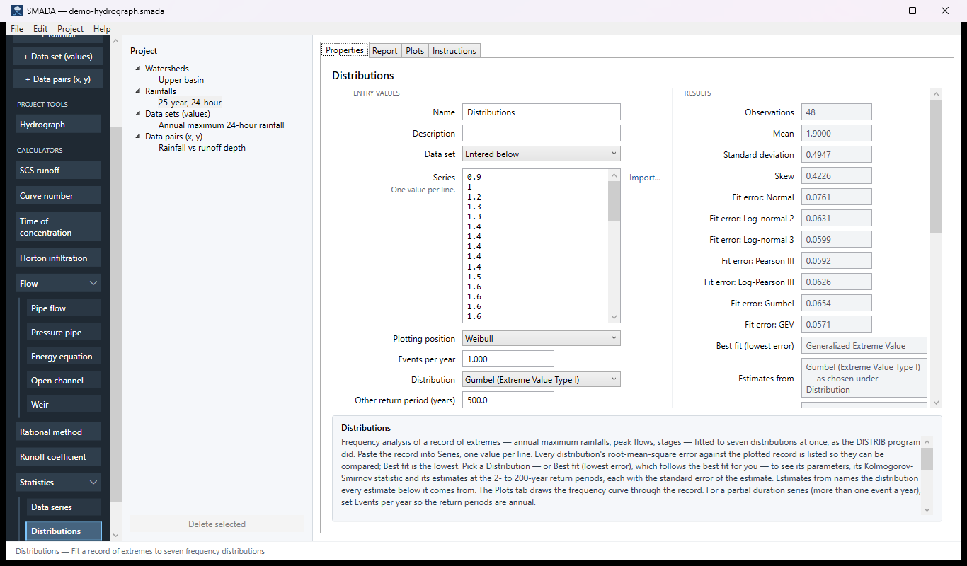
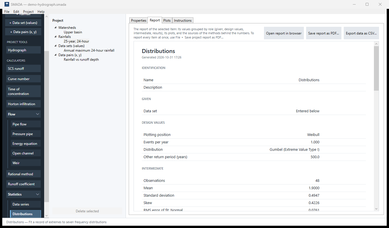
Every item in SMADA has the same four tabs. These are captured from the program with the example values it opens with; select a picture to see it full size.
Properties tab — where you enter values and read the results
Report tab — the same values as a report, ready for HTML, PDF or CSV
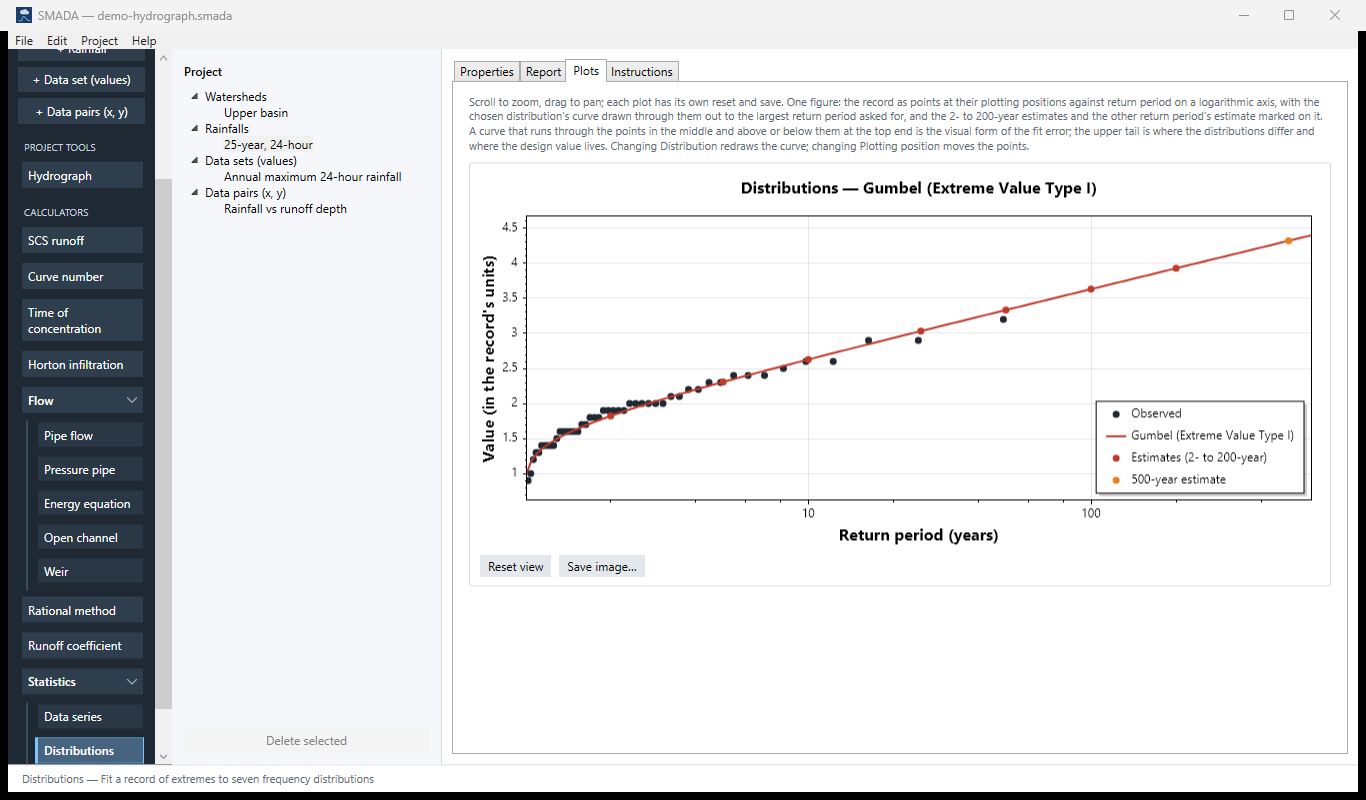
Plots tab — what it draws
Instructions tab — the manual page in the program

How it calculates
Every fit works on the record in its own units; SMADA does not convert it. On each recalculation the record is sorted in ascending order (rank i = 1 is the smallest), the plotting positions are assigned, all seven distributions are fitted and compared (which names the best fit), and then the estimates are written for the distribution chosen under Distribution, or for the best fit when Best fit (lowest error) is chosen. The fits are DISTRIB 2.20's, with the deliberate corrections listed at the end.
1. Sample moments
All fits start from the same three statistics the Data series calculator shows.
x̄ = (1 / n) Σ xi
s = √( Σ (xi − x̄)2 / (n − 1) )
g = n Σ (xi − x̄)3 / ( (n − 1)(n − 2) s3 )
- xi
- the record, sorted ascending, in its own units
- n
- number of values
- x̄
- mean
- s
- sample standard deviation (n − 1 in the denominator)
- g
- unbiased sample skew coefficient (G1), dimensionless
2. Return period and probability
Every estimate is made at a non-exceedance probability p. For a return period T in years and λ events per year:
p = 1 − 1 / (λ T)
- p
- non-exceedance probability, kept between 10−9 and 1 − 10−9
- T
- return period, years
- λ
- Events per year: 1 for an annual series; events in the record divided by years of record for a partial duration series
The standard normal variate z for a probability p (used by the normal, log-normal and Pearson fits) is found by Acklam's rational approximation, relative error about 1.15 × 10⁻⁹.
3. Plotting positions
Each sorted value is given a non-exceedance probability by the formula chosen in Plotting position. The positions are used for the fit-error comparison and the plot; they do not change any fitted parameter.
| Formula | pi for rank i of n (rank 1 smallest) |
|---|---|
| Weibull (default) | i / (n + 1) |
| California | i / n |
| Hazen (Foster) | (2i − 1) / (2n) |
| Cunnane | (i − 0.4) / (n + 0.2) |
| Gringorten | (i − 0.44) / (n + 0.12) |
Every position is kept between 10−6 and 1 − 10−6, so the California formula's largest value (p = 1) stays finite. On the plot a value's return period is 1 / (1 − pi) divided by λ.
4. Normal
xT = x̄ + z s
Standard error of the estimate (Kite's expression for the normal):
ST = s √( (1 + z2/2) / n )
- xT
- estimate with non-exceedance probability p, in the record's units
- z
- standard normal variate for p
- ST
- standard error of xT, in the record's units
Reported parameters: μ = x̄, σ = s.
5. Log-normal, 2 parameter
Fitted to the moments of the record itself (not of its logarithms) by Chow's frequency factor. Every value must be positive: the formulas below would give a number for any record, but a log-normal distribution has no zero or negative values, so a record that has one is not fitted.
Cv = s / x̄
σy2 = ln(1 + Cv2)
μy = ln x̄ − σy2 / 2
K = ( exp(σy z − σy2/2) − 1 ) / Cv
xT = x̄ + K s
Standard error (Kite's expression, first-order with K held fixed):
δ = √( 1 + (Cv3 + 3Cv) K + (Cv8 + 6Cv6 + 15Cv4 + 16Cv2 + 2) K2 / 4 )
ST = δ s / √n
- Cv
- coefficient of variation of the record, dimensionless
- μy, σy
- mean and standard deviation of ln x implied by the moments
- K
- frequency factor, dimensionless
- δ
- standard-error factor, dimensionless
6. Log-normal, 3 parameter
The lower bound a is found from the skew, and x − a is then a two-parameter log-normal. The record must have positive skew.
w = ( −g + √(g2 + 4) ) / 2
z2 = (1 − w2/3) / w1/3
a = x̄ − s / z2
σy = √( ln(z22 + 1) )
μy = ln(s / z2) − σy2 / 2
K = ( exp(σy z − σy2/2) − 1 ) / z2
xT = x̄ + K s
- w, z2
- intermediate quantities from the skew; z2 is the coefficient of variation of x − a
- a
- lower bound of the distribution, in the record's units
- μy, σy
- mean and standard deviation of ln(x − a)
The standard error is DISTRIB's first-order (delta-method) variance, propagated through the first three sample moments: the variances and covariances of m1, m2 and m3 are computed from the fitted distribution's fourth, fifth and sixth central moments, and the partial derivatives of xT with respect to m2 and m3 are taken through w, z2 and K.
ST2 = Var(m1) + Var(m2)(∂x/∂m2)2 + Var(m3)(∂x/∂m3)2 + 2(∂x/∂m2)Cov(m1,m2) + 2(∂x/∂m3)Cov(m1,m3) + 2(∂x/∂m2)(∂x/∂m3)Cov(m2,m3)
- m1, m2, m3
- mean, variance (s2) and third central moment (g s3) of the record
If the computed variance is not positive, no standard error is shown.
7. Pearson Type III
Fitted by moments. The sample skew is first given DISTRIB's small-sample correction (Hazen's factor), and the frequency factor is Kite's series expansion in the corrected skew. The series is an approximation to the exact Pearson Type III frequency factor: it was checked against the Wilson-Hilferty transformation but is not that transformation itself.
g̃ = g (1 + 8.5 / n)
k = g̃ / 6
K = z + (z2 − 1) k + (z3 − 6z) k2/3 − (z2 − 1) k3 + z k4 + k5/3
xT = x̄ + K s
Standard error (Kite):
δ2 = 1 + g̃K + (1 + 0.75 g̃2) K2/2 + 3K (∂K/∂g)(g̃ + 0.25 g̃3) + 3(∂K/∂g)2(2 + 3g̃2 + 5g̃4/8)
ST = √( s2 δ2 / n )
- g̃
- skew after the (1 + 8.5/n) correction, dimensionless
- K
- Pearson III frequency factor
- ∂K/∂g
- slope of the series with respect to skew, differentiated term by term
Reported parameters: the mean, standard deviation and corrected skew, and
β = (2 / g̃)2
α = sign(g̃) s / √β
γ = x̄ − αβ
- β
- shape, dimensionless
- α
- scale, in the record's units; it carries the sign of the skew
- γ
- location, in the record's units: the lower bound x̄ − s√β for positive skew, the upper bound x̄ + s√β for negative skew
With these signs the three parameters give back the mean (γ + αβ), the standard deviation (|α|√β) and the corrected skew. They are reported only; the estimates come from the frequency factor. A record with zero skew is not fitted; Pearson III is then the normal distribution.
8. Log-Pearson Type III
The same Pearson III fit, made on y = ln x (natural logarithms), by the method of moments in log space: the distribution and fitting method of Bulletin 17B. It is not a full Bulletin 17B analysis. As DISTRIB did, the station skew of the logarithms carries the small-sample factor (1 + 8.5/n), which Bulletin 17B does not use; the skew is not weighted with a regional (generalized) skew; and there are no tests for high or low outliers. Every value must be positive.
yT = ȳ + K sy
xT = exp(yT)
- ȳ, sy
- mean and standard deviation of ln x
- K
- Kite's series in the corrected skew of ln x
The standard error Sy is the Pearson expression above, in log units. Back in real units the error is not symmetric, so the two one-sided errors are averaged, as DISTRIB reported it:
ST = [ xT(eSy − 1) + xT(1 − e−Sy) ] / 2
Log-Pearson is not fitted if any value is zero or negative, or if the logarithms have zero skew (it is then the two-parameter log-normal).
9. Gumbel (Extreme Value Type I)
Gumbel's small-sample method: the reduced variate is standardised by its own mean and standard deviation for a sample of this size, rather than by the large-sample constants. The reduced variates are always taken at Weibull positions i/(n + 1), whatever Plotting position is set to.
yi = −ln( −ln( i / (n + 1) ) ), i = 1 … n
ȳn = (1/n) Σ yi
σn = √( (1/n) Σ yi2 − ȳn2 )
K = ( −ln(−ln p) − ȳn ) / σn
xT = x̄ + K s
Standard error (Kite):
ST = s √( (1 + 1.1396 K + 1.1 K2) / n )
- yi
- reduced variate at rank i
- ȳn, σn
- mean and standard deviation of the reduced variates for n values (for n = 20, σn = 1.0628, Gumbel's table)
Reported parameters: scale α = σn / s (shown as 1/α), mode u = x̄ − ȳn/α, and ȳn and σn. As n grows, K tends to the large-sample factor used by the Data series calculator.
10. Generalized extreme value (GEV)
Fitted by L-moments (probability-weighted moments), with the shape from the L-skewness by Hosking's approximation. It needs at least four values.
b0 = (1/n) Σ xi
b1 = (1/n) Σ [ (i − 1) / (n − 1) ] xi
b2 = (1/n) Σ [ (i − 1)(i − 2) / ((n − 1)(n − 2)) ] xi
λ1 = b0, λ2 = 2b1 − b0, λ3 = 6b2 − 6b1 + b0, τ3 = λ3 / λ2
c = 2 / (3 + τ3) − ln 2 / ln 3
k = 7.8590 c + 2.9554 c2
α = λ2 k / ( (1 − 2−k) Γ(1 + k) )
ξ = λ1 − α (1 − Γ(1 + k)) / k
xT = ξ + α (1 − (−ln p)k) / k
- xi
- the record sorted ascending, rank i
- b0, b1, b2
- probability-weighted moments
- λ1, λ2, λ3
- first three L-moments
- τ3
- L-skewness
- k
- shape: k > 0 bounded above (Weibull type), k < 0 heavy upper tail (Fréchet type)
- α, ξ
- scale and location, in the record's units
- Γ
- gamma function, by the Lanczos approximation
When |k| < 10−8 the Gumbel limit is used: α = λ2 / ln 2, ξ = λ1 − 0.5772 α, xT = ξ − α ln(−ln p). The GEV has no standard error, as in DISTRIB; the published one needs the full covariance of the L-moment estimators.
11. Comparing the fits
For every distribution that can be fitted, the Fit error is the root-mean-square (RMS) difference between the fitted value and the record at the plotting positions, in the record's units (DISTRIB's measure). Best fit (lowest error) names the smallest. It is a guide, not a verdict: a distribution that cannot be fitted is left out, and in a small record any of them can come out lowest.
RMS = √( (1/n) Σ ( x̂(pi) − xi )2 )
- x̂(pi)
- the fitted distribution's value at the plotting position of rank i
For the chosen distribution, the Kolmogorov-Smirnov statistic is the one-sample D, the largest gap between the record's step-wise cumulative frequency and the fitted distribution, taken on both sides of each step:
D = maxi max( |i/n − F(xi)|, |(i − 1)/n − F(xi)| )
F(x) is found by bisection on the fitted quantile function (80 halvings between p = 10−9 and 1 − 10−9), so the same method serves every distribution, including the Pearson forms, which have no closed-form CDF. Compare D with the critical value for the sample size, about 1.36/√n at the 5 % level for n over 35.
12. The estimates
The Distribution drop-down lists the seven distributions and, first, Best fit (lowest error), which follows whichever distribution has the lowest fit error and changes with the record. Estimates from names the distribution every value below it comes from (its parameters, its Kolmogorov-Smirnov D and its estimates), with "as chosen under Distribution" or "the best fit". It is not necessarily the best fit: compare the Best fit (lowest error) row above it.
For that distribution, xT and ST are written at T = 2, 5, 10, 25, 50, 100 and 200 years, and at the Other return period if it is greater than 1, each at p = 1 − 1/(λT). The standard errors are first-order (Kite 1977): about two thirds of records like this one would put the true value within one standard error. They are approximate for strongly skewed records.
13. The plot
The Plots tab draws the record as points at their plotting positions against return period on a logarithmic axis, with the distribution's curve drawn through them out to the largest return period asked for. The 2- to 200-year estimates and the Other return period estimate are marked on the curve, the legend sits at the lower right, and the title names the distribution, with "(best fit)" when Best fit (lowest error) chose it. Changing Plotting position moves the points; changing Distribution redraws the curve.
When a distribution is not fitted
- Fewer than three values, or every value the same: nothing is fitted.
- Two-parameter log-normal: every value must be positive.
- Three-parameter log-normal: the skew must be positive.
- Pearson Type III: the skew must not be zero.
- Log-Pearson Type III: every value must be positive, and the logarithms must not have zero skew.
- GEV: at least four values.
A distribution that cannot be fitted shows a dash for its fit error and is left out of Best fit; when it is the one chosen, the reason is shown and its estimates are blank. If none can be fitted and Best fit (lowest error) is chosen, Estimates from says so.
Departures from DISTRIB
SMADA's ENGINE-DEPARTURES notes 11 and 17 record these, each held by a test.
- Gumbel: DISTRIB divided by the variance of the reduced variate instead of its standard deviation (about 6 % error in K at n = 20). SMADA uses σn.
- Normal variate: DISTRIB used Abramowitz and Stegun 26.2.23 (error 4.5 × 10⁻⁴); SMADA uses Acklam's approximation.
- Pearson III series: DISTRIB's last term was −k5/3; SMADA follows Kite's printed form, +k5/3. The difference is negligible for |g| < 2, and neither sign is closer to the exact Pearson III factor.
- Normal standard error: DISTRIB used δ2 = 1 + z2; Kite's 1 + z2/2 is used.
- Kolmogorov-Smirnov: DISTRIB computed a two-sample statistic between the record and the fitted quantiles; SMADA computes the one-sample D above.
- Log-Pearson III is fitted by moments of the logarithms only; DISTRIB first tried a real-space fit and fell back to this.
- Two-parameter log-normal: DISTRIB fitted it to any record; SMADA requires every value to be positive.
- Pearson III parameters: DISTRIB always reported a positive α and γ = x̄ − s√β, which do not give back a negative skew; SMADA gives α the sign of the skew. The estimates were not affected.
Checking the example by hand
The calculator opens with DISTRIB's PANAMA.XD2 sample, 48 annual values already in ascending order:
| Ranks | Values |
|---|---|
| 1–12 | 0.9, 1.0, 1.2, 1.3, 1.3, 1.4, 1.4, 1.4, 1.4, 1.4, 1.5, 1.6 |
| 13–24 | 1.6, 1.6, 1.6, 1.6, 1.6, 1.7, 1.7, 1.8, 1.8, 1.8, 1.9, 1.9 |
| 25–36 | 1.9, 1.9, 1.9, 2.0, 2.0, 2.0, 2.0, 2.0, 2.0, 2.1, 2.1, 2.2 |
| 37–48 | 2.2, 2.3, 2.3, 2.4, 2.4, 2.4, 2.5, 2.6, 2.6, 2.9, 2.9, 3.2 |
- The values sum to 91.2, so x̄ = 91.2 / 48 = 1.9000; the sample standard deviation is s = 0.4947 and the skew g = 0.4226.
- Gumbel, 100-year: the reduced variates −ln(−ln(i/49)) for i = 1 … 48 have ȳ48 = 0.5477 and σ48 = 1.1573. At T = 100, p = 0.99 and −ln(−ln 0.99) = 4.6001, so K = (4.6001 − 0.5477) / 1.1573 = 3.502 and x100 = 1.900 + 3.502 × 0.4947 = 3.632. Its standard error is 0.4947 √((1 + 1.1396 × 3.502 + 1.1 × 3.5022) / 48) = 0.307.
- The mode is u = x̄ − ȳ48 s / σ48 = 1.9 − 0.5477 × 0.4947 / 1.1573 = 1.6659, and the scale 1/α = s / σ48 = 0.4274, as the Parameters line shows.
- The same steps give the other Gumbel estimates: 1.823 at 2 years, 2.307 at 5, 2.628 at 10, 3.033 at 25, 3.334 at 50, 3.929 at 200 and 4.322 at the 500-year Other return period, the points marked on the plot.
- The seven fit errors on the form run from 0.0571 for the GEV, named Best fit (lowest error), to 0.0761 for the normal; the Gumbel, which Estimates from names "as chosen under Distribution", has 0.0654 and a Kolmogorov-Smirnov D of 0.1025.
Every fit, fit error, D and standard error was also checked against independent references: scipy for the quantiles, the Kolmogorov-Smirnov statistic and the fit errors; Gumbel's table of ȳn and σn; and the Bulletin 17B Appendix 3 table of Pearson frequency factors, which Kite's series matches to within 0.0125 in K for skews up to ±1.
Sources
- Eaglin, R. and Wanielista, M., DISTRIB 2.20, Statistical Distribution Analysis, University of Central Florida, 1992–2001.
- Kite, G. W., Frequency and Risk Analyses in Hydrology, Water Resources Publications, 1977 (Chapters 5–10: normal, two- and three-parameter log-normal, Pearson Type III, log-Pearson Type III, Gumbel).
- Chow, V. T., 'The log-probability law and its engineering applications', Proc. ASCE 80, 1954.
- U.S. Interagency Advisory Committee on Water Data, Bulletin 17B, Guidelines for Determining Flood Flow Frequency, 1982.
- Gumbel, E. J., Statistics of Extremes, Columbia University Press, 1958.
- Hosking, J. R. M., Wallis, J. R. and Wood, E. F., 'Estimation of the generalized extreme-value distribution by the method of probability-weighted moments', Technometrics 27(3), 1985.
All SMADA calculators · Get SMADA free for Windows from the Microsoft Store