Data series
The mean, standard deviation and skew of a record of annual maxima, and the Gumbel estimate of the event with a chosen return period.
What it is for
Data series is the first look at a record of extremes: the largest daily rainfall of each year, the annual peak flow at a gauge, the annual high stage of a lake. It answers two questions. What does the record look like (its size, center, spread and lopsidedness)? And how large is the event you can expect, on average, once in T years?
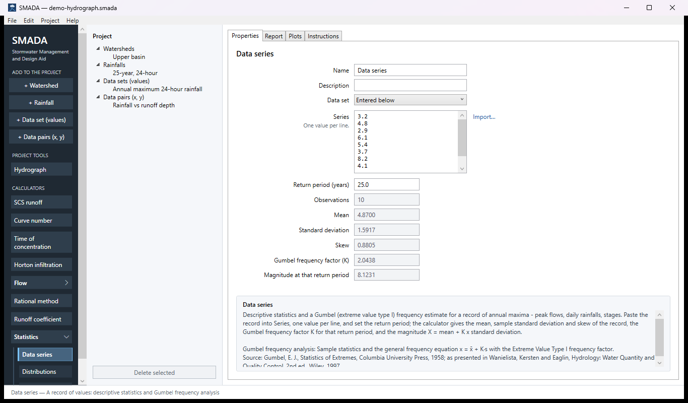
You enter the record, one value per line, either typed or pasted into Series (leave Data set at Entered below) or taken from a data set you have added to the project with + Data set (values). You set Return period (years). SMADA gives back the number of observations, the mean, the sample standard deviation and the skew of the record, the Gumbel frequency factor K for your return period, and the magnitude X = mean + K × standard deviation, in the units of the record.
It assumes the Gumbel (Extreme Value Type I) distribution and uses the large-sample frequency factor, which is the quickest frequency estimate there is. When the choice of distribution is itself the question, or you want the whole 2- to 200-year table with standard errors, use the Distributions calculator, which reads the same data sets and fits seven distributions at once.
The Data series tabs
Every item in SMADA has the same four tabs. These are captured from the program with the example values it opens with; select a picture to see it full size.
Data series has nothing to draw, so its Plots tab is empty and is not shown.
Properties tab — where you enter values and read the results
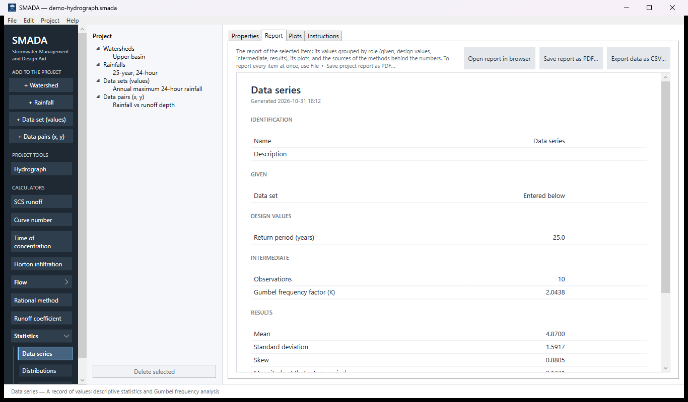
Report tab — the same values as a report, ready for HTML, PDF or CSV
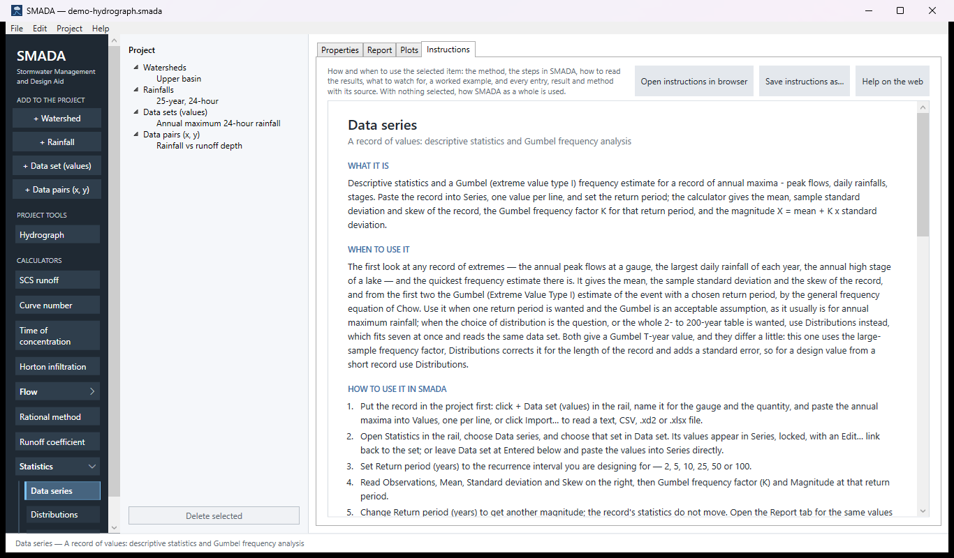
Instructions tab — the manual page in the program
How it calculates
The calculator works on the values exactly as entered, in their own units; SMADA does not convert a data series. The order of the values does not matter. Every result is recomputed whenever the series or the return period changes.
1. Reading the record
If a project data set is chosen in Data set, its values are copied into Series and locked; otherwise the values typed into Series are used. The report names the data set, or says Entered below when the values were typed in. Observations is the count n of values read.
2. Mean
x̄ = (1 / n) Σ xi
- x̄
- arithmetic mean of the record, in the record's units
- xi
- the i-th value of the record
- n
- number of values
3. Sample standard deviation
The sample form is used, with n − 1 in the denominator, not the population form with n.
s = √( Σ (xi − x̄)2 / (n − 1) )
- s
- sample standard deviation, in the record's units
4. Skew
The skew is the sample coefficient of skewness with the usual small-sample unbiasing factor (the G1 form, the same one spreadsheets report as SKEW). It uses the sample standard deviation s from step 3.
g = n Σ (xi − x̄)3 / ( (n − 1)(n − 2) s3 )
- g
- sample skew coefficient, dimensionless; positive for a long tail of large values
If every value is the same (s = 0) the skew is reported as 0.
5. Gumbel frequency factor
The frequency factor for the Gumbel (Extreme Value Type I) distribution is the large-sample (asymptotic) form. It depends only on the return period, not on the record.
K = −(√6 / π) [ 0.5772 + ln( ln( T / (T − 1) ) ) ]
- K
- Gumbel frequency factor, the number of standard deviations above the mean, dimensionless
- T
- return period, years (must be greater than 1)
- 0.5772
- Euler's constant; the code carries it to full precision, 0.5772156649
Some reference values: K ≈ −0.164 at T = 2 years (the Gumbel median lies a little below the mean), 2.044 at 25 years, 3.137 at 100 years.
6. Magnitude at the return period
The estimate follows the general frequency equation of Chow.
XT = x̄ + K s
- XT
- magnitude of the event with return period T, in the record's units
The annual exceedance probability of XT is 1 / T.
Limits and checks
- With no values every result is 0.
- With one value only the mean is given; standard deviation, frequency factor and magnitude stay 0.
- With fewer than three values the skew stays 0.
- A return period of 1 year or less leaves K and the magnitude at 0.
- The skew is reported but does not enter the Gumbel estimate, which uses only the mean and the standard deviation. A Gumbel distribution has a skew of about 1.14; a record far from that is a hint that another distribution may fit better.
- Because K is the large-sample form, the estimate runs a little low for short records. The Gumbel in the Distributions calculator corrects K for the sample size (Gumbel's ȳn and σn) and gives a standard error with each estimate. For this calculator's ten-value example the 100-year value is 9.86 here and 11.75 in Distributions; both are right for their method. For a design value from a short record, or when the choice of distribution is the question, use Distributions.
Checking the example by hand
The calculator opens with ten values: 3.2, 4.8, 2.9, 6.1, 5.4, 3.7, 8.2, 4.1, 5.9, 4.4, and T = 25 years. The sum is 48.7, so x̄ = 4.87. The squared deviations sum to 22.801, so s = √(22.801 / 9) = 1.5917. The skew is 0.8805. K for 25 years is −(√6 / π)[0.5772 + ln(ln(25/24))] = −0.7797 × (0.5772 − 3.1985) = 2.0438, and X25 = 4.87 + 2.0438 × 1.5917 = 8.1231, as the form shows. Each of these statistics was also checked against numpy and scipy, and K against the table in Chow, Maidment and Mays (2.044 at 25 years).
Sources
- Gumbel, E. J., Statistics of Extremes, Columbia University Press, 1958; as presented in Wanielista, Kersten and Eaglin, Hydrology: Water Quantity and Quality Control, 2nd ed., Wiley, 1997.
All SMADA calculators · Get SMADA free for Windows from the Microsoft Store