Watershed
Holds a drainage area's size, directly connected impervious area, time of concentration and loss method, and turns each step of a storm into excess rainfall for the Hydrograph tool, weighting the connected and unconnected parts by area as TR-55 does.
What it is for
A watershed is the land that drains to one outlet. Before you can ask how much runoff a storm makes, you have to say how big that land is, how much of it is paved and piped straight to the outlet, how long water takes to cross it, and how much of the rain the ground keeps. The Watershed item in SMADA holds those answers; it is the first thing a project needs.
You enter the Total area, the Impervious area and the Directly connected impervious area (DCIA), the Time of concentration (typed, or brought back from the Time of concentration calculator with Calculate…), and a small Additional abstraction, impervious for the connected pavement. Then you choose a Loss method, Curve number, Horton or Constant rate, and fill in its parameters, which appear under the drop-down. Under Curve number the watershed shows one derived value, the Initial abstraction (Ia) = 0.2 S. The three areas are checked against each other: the DCIA must be no larger than the impervious area, and that no larger than the total; a red note says so when they are not.
A watershed does not hold the rain and does not draw a hydrograph by itself. The Hydrograph tool combines it with a Rainfall: the DCIA and the rest of the watershed each receive the whole storm, the loss method decides what the part that is not directly connected keeps, and the two runoff depths are weighted by area, as TR-55 does. The Hydrograph tool then turns that excess into flow. Use one watershed per drainage area and condition; pre-development and post-development are two watersheds, not one edited twice.
The Watershed tabs
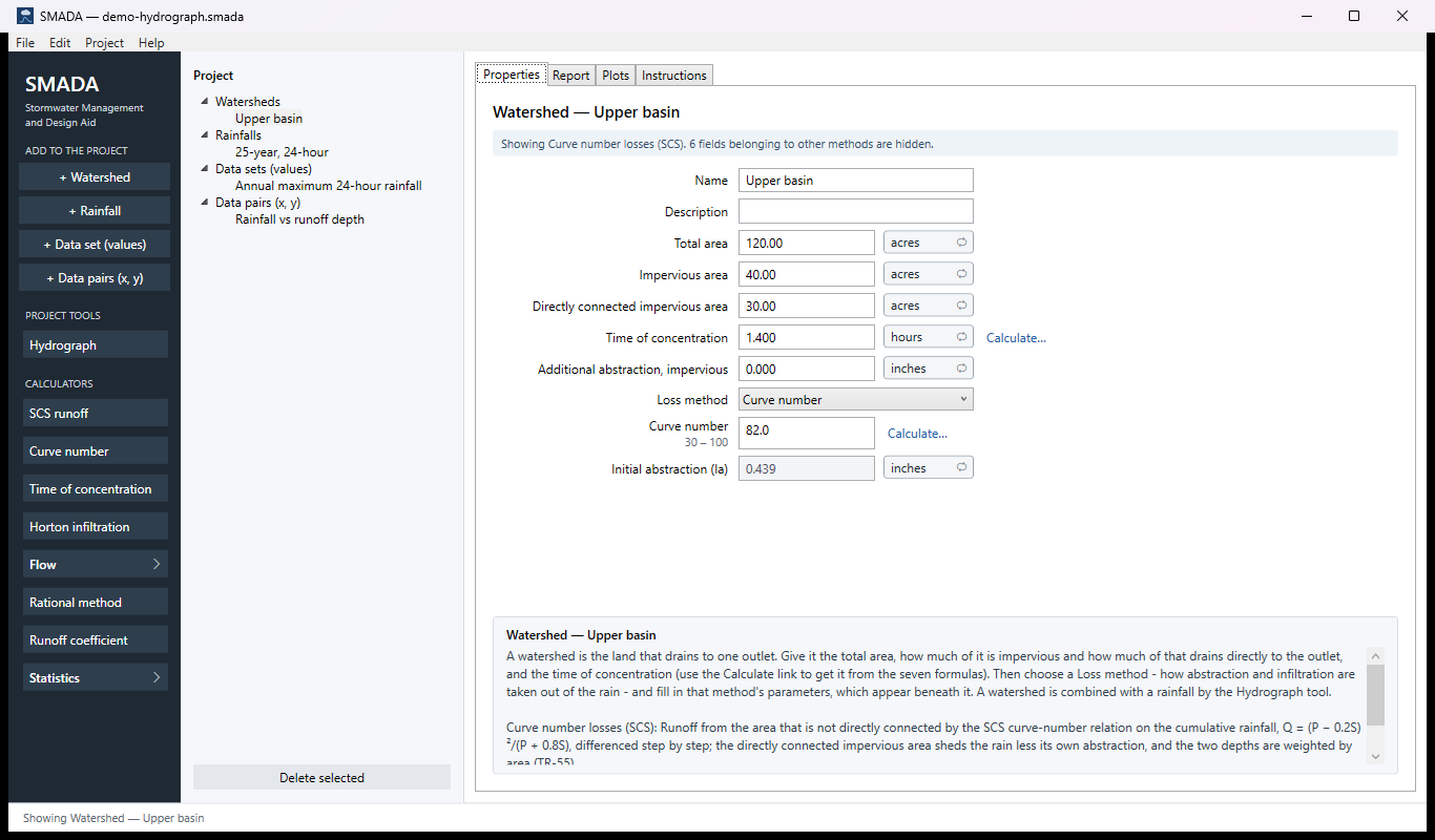
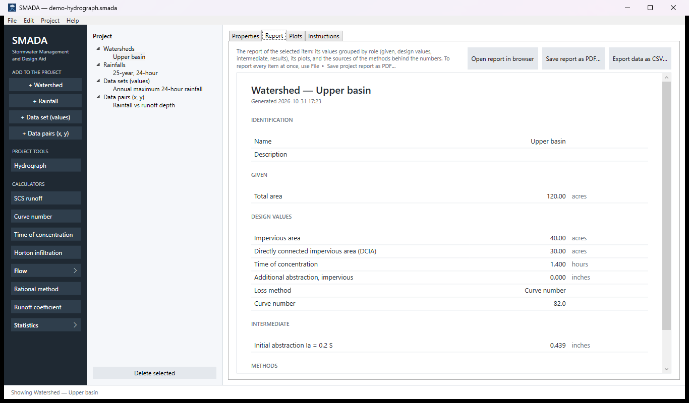
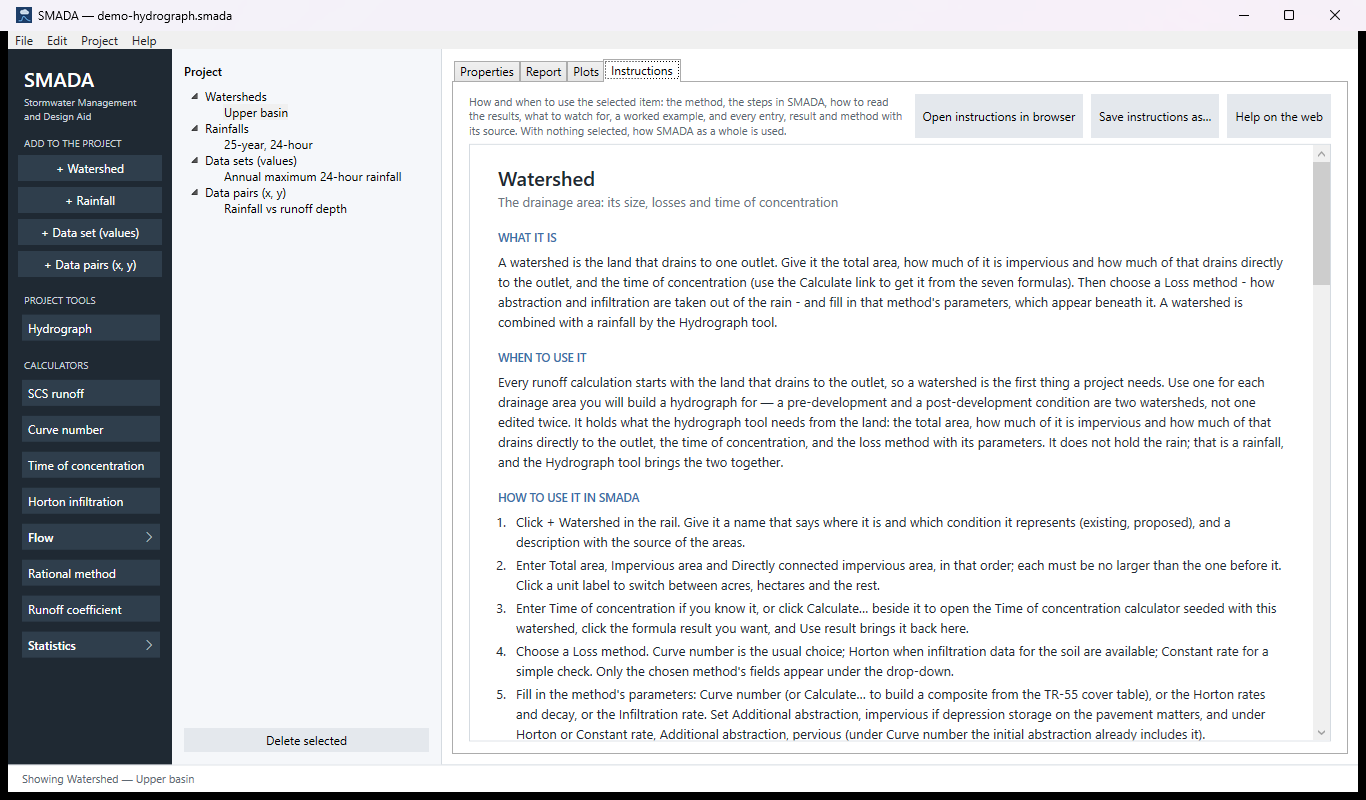
Every item in SMADA has the same four tabs. These are captured from the program with the example values it opens with (and the demo project's watershed and rainfall); select a picture to see it full size.
Watershed has nothing to draw, so its Plots tab is empty and is not shown.
Download the example project (demo-hydrograph.smada: the watershed Upper basin, the 25-year, 24-hour rainfall and two data sets) and open it in SMADA with File ▸ Open to see these same numbers.
Properties tab — where you enter values and read the results
Report tab — the same values as a report, ready for HTML, PDF or CSV
Instructions tab — the manual page in the program
How it calculates
On its own a watershed computes one value: the initial abstraction under the curve number method. Its real work happens when the Hydrograph tool runs: the loss method is handed the rainfall depth of each computation step and returns the excess rainfall for each step, in inches over the whole watershed. Depths below are inches, times are hours.
What is stored, and what is checked
Total area, impervious area and DCIA are stored in acres; time of concentration in hours; abstractions and maximum infiltration in inches; the infiltration rate and the Horton rates in inches per hour (click the unit label to enter them in cm/hr or mm/hr); the Horton decay k is always per hour. The form reports any value outside its declared range (all of them at least 0; curve number 30 to 100) rather than changing it. The time of concentration is a stored number, not a formula: the Time of concentration calculator can hand its result to it.
A red note above the form, and a refusal in the Hydrograph tool, follow from these checks:
- the impervious area is larger than the total area;
- the DCIA is larger than the impervious area (it is part of it), or, when the impervious area is left at 0, larger than the total area. An impervious area of 0 is not itself checked, so you can leave it at 0 if you know only the DCIA;
- under Horton, k is not greater than 0, or the initial rate fo is below the final rate fc.
The Hydrograph tool also will not run a watershed whose total area or time of concentration is zero.
Splitting off the directly connected impervious area
Every loss method starts the same way. The watershed is divided into its directly connected impervious area and the rest:
fd = DCIA / A (limited to 0 … 1), fp = 1 − fd
- fd
- directly connected impervious fraction, dimensionless
- fp
- the rest of the watershed, dimensionless
- DCIA
- directly connected impervious area, acres
- A
- total area, acres
Both parts receive the whole rainfall, and each produces a runoff depth over its own area. The watershed's excess in step k is the area-weighted sum:
Ek = fd Ed,k + fp Ep,k
- Ek
- excess rainfall in step k, in over the whole watershed
- Ed,k
- runoff from the directly connected impervious area in step k, in over that area
- Ep,k
- runoff from the rest in step k, in over that area, by the loss method chosen
This is TR-55's weighting (Chapter 2): the connected pavement and the rest each see the full storm, and their runoff depths are combined by area. Until 2026-10-15 SMADA instead scaled the rain to fp P and took the full abstraction and infiltration from that, which overstated the losses; the example below gave 6.553 in of runoff that way, where TR-55 gives 6.973 in.
Only the DCIA enters the arithmetic. Impervious area that is not directly connected (roofs and drives draining onto lawns) is not used separately: as in TR-55 it belongs in the composite curve number, counted at CN 98, or in the infiltration parameters. The Impervious area is checked against the other two areas and reported, nothing more. For the same reason the Curve number calculator, opened with Calculate… from a watershed, covers the total area less the DCIA.
The directly connected impervious area
The connected pavement sheds each step's rain after the impervious abstraction is used up. The abstraction is taken from the first rain:
ak = min(Rd, Pk), Rd ← Rd − ak
Ed,k = Pk − ak
- Pk
- rainfall in step k, in
- Rd
- impervious abstraction still to be filled, starting at Additional abstraction, impervious, in
- ak
- abstraction taken in step k, in
This applies under every loss method.
Curve number
The potential maximum retention and the initial abstraction follow from the curve number:
S = 1000 / CN − 10
Ia = 0.2 S
Ia is the value shown, locked, on the form as Initial abstraction (Ia). The runoff relation is applied to the cumulative rainfall and differenced step by step:
Pc,k = P1 + P2 + … + Pk
Q(P) = (P − 0.2 S)2 / (P + 0.8 S) for P > 0.2 S; Q(P) = 0 otherwise
Ep,k = Q(Pc,k) − Q(Pc,k−1)
- CN
- curve number of all the area that is not directly connected, 30 to 100
- S
- potential maximum retention, in
- Ia
- initial abstraction, in
- Pc,k
- cumulative rainfall to the end of step k, in
- Q(P)
- cumulative runoff depth, in
- Ep,k
- runoff from the area that is not directly connected in step k, in over that area
Working from the cumulative curve is what makes the increments add up to the storm's runoff; applying the relation to each step separately would subtract the initial abstraction again at every step.
Additional abstraction, pervious is not offered under this method: TR-55's Ia = 0.2 S already includes surface storage, so adding to it would count it twice.
Horton
Horton's capacity falls from an initial rate toward a final rate, and its integral is the depth a ponded soil takes in by time t:
f(t) = fc + (fo − fc) e−k t
F(t) = fc t + (fo − fc) (1 − e−k t) / k
During a storm the soil takes only what the rain delivers, so the clock that matters is not the storm's but the depth actually infiltrated so far, F. SMADA finds the equivalent time t* at which a ponded soil would have taken in F, by bisection on F(t*) = F (the upper bound starts at 1 hr and doubles until F(t) passes F; then halving until the bracket is narrower than 10−10 hr, at most 200 times). The capacity over the step is Horton's own integral from there:
Ck = F(t* + Δt) − F(t*)
Each step k then does:
- available depth: d = Pk, the whole step's rain;
- pervious abstraction, taken from the first rain: b = min(Rp, d), Rp ← Rp − b, d ← d − b;
- room left under the cap: H = max(Fmax − F, 0), with no cap when Fmax = 0;
- infiltration in the step: ΔF = min(Ck, d, H);
- F ← F + ΔF, and the step's runoff is Ep,k = d − ΔF.
- fo
- Horton initial rate, in/hr
- fc
- Horton final rate, in/hr
- k
- Horton decay, per hour
- F
- depth infiltrated so far, in
- t*
- equivalent time: when a ponded soil would have taken in F, hr
- Ck
- infiltration capacity over step k, in
- Rp
- pervious abstraction still to be filled, starting at Additional abstraction, pervious, in
- Fmax
- Maximum infiltration, in (0 means no cap)
- Δt
- computation step, hr
Under ponding this gives exactly Horton's F(t) at any step. Until 2026-10-15 SMADA took the rate at the start of each step times Δt, which ignored the decay within the step: ponded for two hours at fo = 3, fc = 0.5, k = 4 it infiltrated 9 % more than F(2) at a 0.25 hr step and 39 % more at 0.5 hr. Projects with Horton losses now show less infiltration and more runoff. SMADA 10 before that solved for the rate by a stepping search that returned fc when it gave up after 50 tries; the bisection always converges.
The Horton recovery (kr) value is no longer offered. Recovery of capacity happens between storms, and SMADA runs one storm, so the value is kept in files that carry it but has no effect on any result.
Constant rate
The same steps as Horton with a fixed rate:
ΔF = min(fr Δt, d, H)
Ep,k = d − ΔF
- fr
- Infiltration rate, in/hr (negative values taken as 0)
- d
- the step's rain left after the pervious abstraction, in
- H
- room left under the maximum infiltration, in
- ΔF
- depth infiltrated in the step, in
Under both infiltration methods the rate applies at its full value to the area that is not directly connected; before 2026-10-15 the rain was scaled by fp first, so these methods took 1/fp too much.
Checking the example by hand
In the example project, Upper basin is 120 acres with 30 acres directly connected, so fd = 30 / 120 = 0.25 and fp = 0.75. With CN = 82:
S = 1000 / 82 − 10 = 2.195 in, Ia = 0.2 × 2.195 = 0.439 in
which is the Initial abstraction the form shows. For the 8.6 in storm with no impervious abstraction, the connected 30 acres shed all 8.6 in. The other 90 acres also receive 8.6 in and, by the curve number,
Q(8.6) = (8.6 − 0.439)2 / (8.6 + 0.8 × 2.195) = 8.1612 / 10.356 = 6.431 in
Because SMADA differences the cumulative curve, the per-step increments add to this whatever the storm's pattern. Weighted by area,
E = 0.25 × 8.6 + 0.75 × 6.431 = 2.150 + 4.823 = 6.973 in
and the losses are 8.6 − 6.973 = 1.627 in, which is what the Hydrograph tool reports for this watershed (Runoff depth 6.973 in, Losses 1.627 in).
Sources
- USDA NRCS, National Engineering Handbook, Part 630 Hydrology, Chapter 10, 2004 (curve number losses).
- USDA SCS, Technical Release 55, Urban Hydrology for Small Watersheds, 2nd ed., 1986, Chapter 2 (curve number losses and the area weighting used by all three methods).
- Horton, R. E., Soil Science Society of America Proceedings 5, 1940 (Horton losses).
- Wanielista, Kersten and Eaglin, Hydrology: Water Quantity and Quality Control, 2nd ed., Wiley, 1997 (constant-rate losses).
All SMADA calculators · Get SMADA free for Windows from the Microsoft Store