Rainfall
A design storm as depths against time, typed in or generated from a total depth, a storm duration and a published dimensionless mass curve such as the NRCS TR-20 Type II table.
What it is for
A rainfall in SMADA is a design storm: how much rain falls, over how long, and in what pattern through the storm. It is not a calculator in the list of tools down the left side of SMADA but a project item, added with + Rainfall, and you keep one for each event you want to run, such as a 25-year 24-hour storm for a pond or a 10-year 1-hour storm for a pipe.
You make one in either of two ways, chosen with Method. Under Entered you set a Time step and paste the depth that falls in each step, one per line, when you already have a recorded or published hyetograph; SMADA then derives the Total depth and the Series duration. Under Dimensionless curve you pick a published mass curve, enter the total depth from the rainfall atlas and the Storm duration, and SMADA generates the depths for you. The SCS Type I, IA, II and III curves are the NRCS TR-20 rainfall tables; the Type II Florida Modified and Florida DOT curves (1 to 240 hours) are still the archived SMADA 5 storms, not yet re-checked against the current FDOT Drainage Manual, and SMADA says so beside each one.
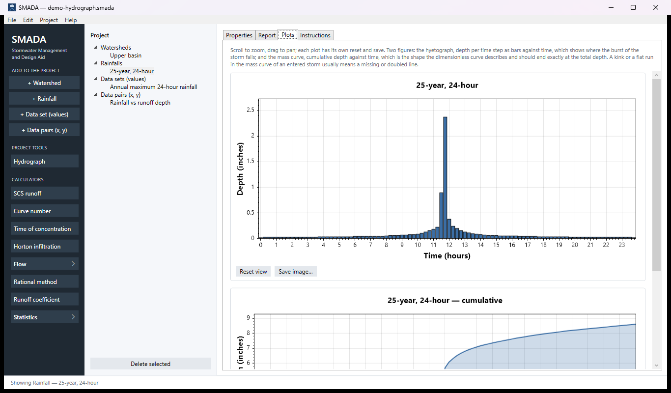
What you get back is the series of incremental depths, its total and duration, and on the Plots tab two figures: the hyetograph (depth per step) and the mass curve (cumulative depth). The report lists the values and the figures, and the depths can be exported as CSV.
A rainfall does nothing on its own. The Hydrograph tool pairs it with a watershed, takes off the losses (for example by the SCS curve number) and turns the excess into a runoff hydrograph. The Hydrograph tool resamples the storm onto its own computation step, so the rainfall's time step need not match it.
The Rainfall tabs
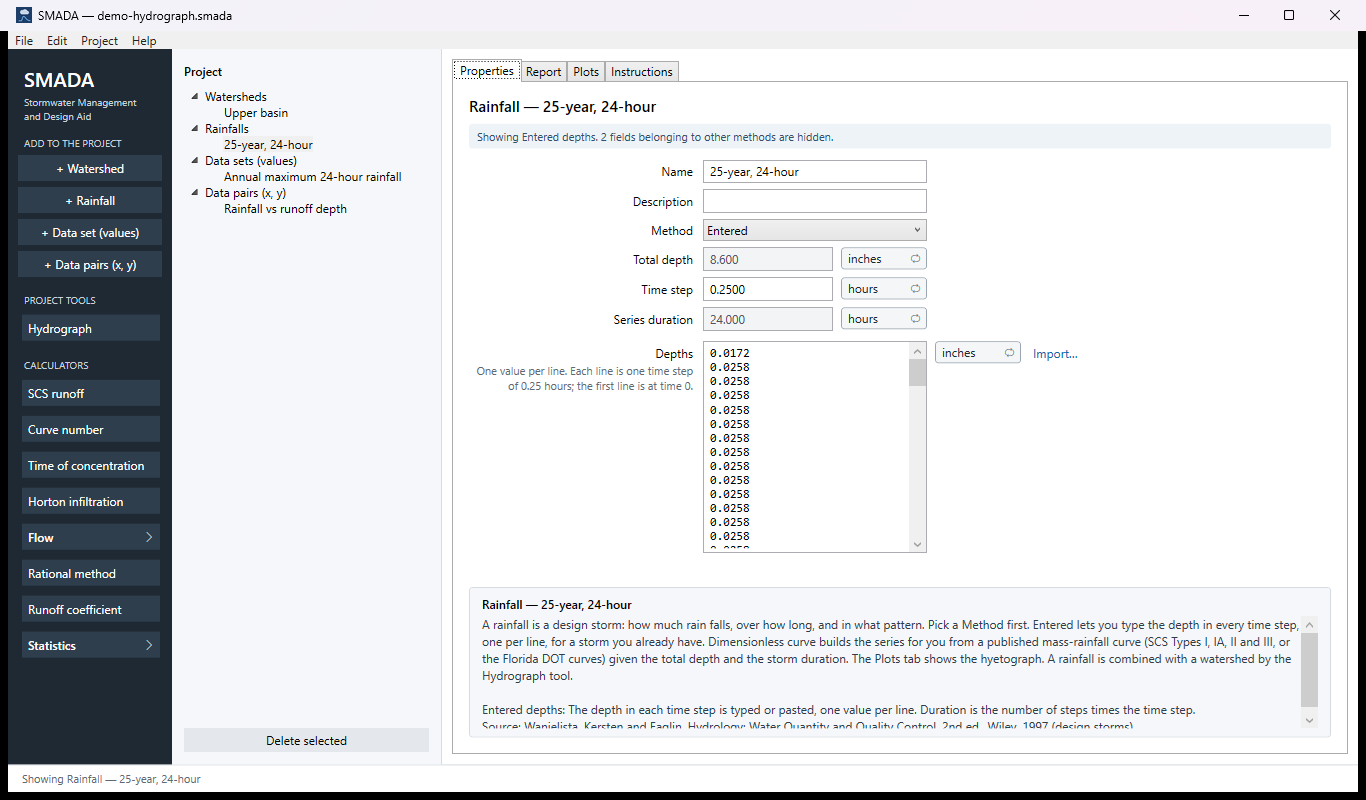
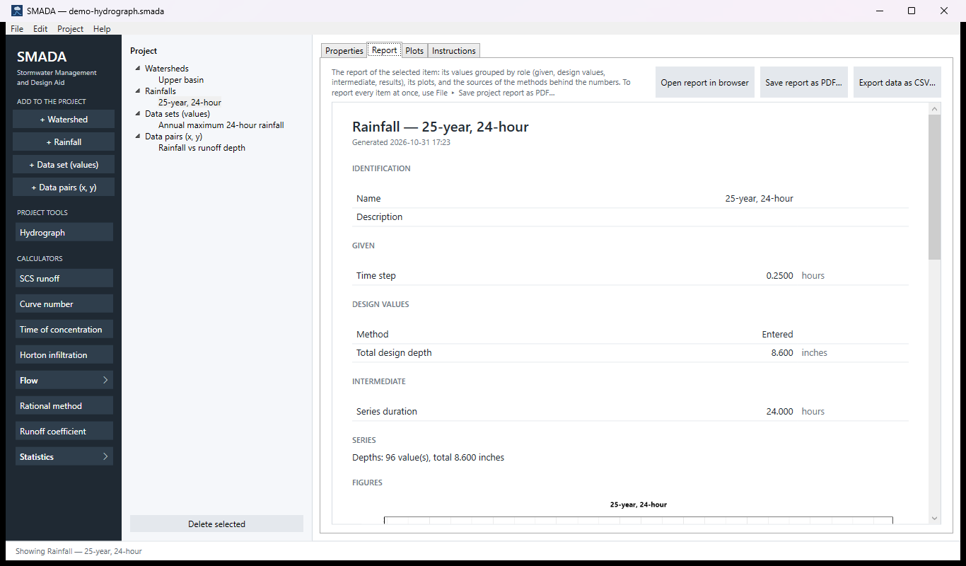
Every item in SMADA has the same four tabs. These are captured from the program with the example values it opens with (and the demo project's watershed and rainfall); select a picture to see it full size.
Download the example project (demo-hydrograph.smada: the watershed Upper basin, the 25-year, 24-hour rainfall and two data sets) and open it in SMADA with File ▸ Open to see these same numbers.
Properties tab — where you enter values and read the results
Report tab — the same values as a report, ready for HTML, PDF or CSV
Plots tab — what it draws
Instructions tab — the manual page in the program
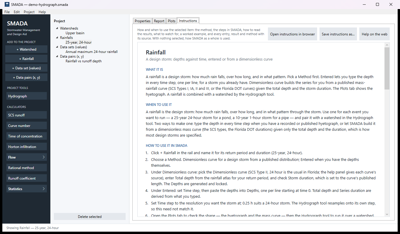
How it calculates
A rainfall is stored as a series of incremental depths, one per time step, in inches, with times in hours. The first depth is the rain in the step that starts at time 0. The Method decides how that series comes to be, and the form shows only the fields that method uses.
Entered depths
You set the Time step Δt and type or paste the Depths. There is nothing to solve; SMADA derives two values from the series so they cannot disagree with it:
P = Σ pi
Ds = n × Δt
- P
- total depth of the storm, in (shown as Total depth, locked under this method)
- pi
- depth that falls in step i, in
- n
- number of depths entered
- Δt
- time step, hr
- Ds
- how long the series runs, hr (shown as Series duration)
- A pasted line that is not a number rejects the whole paste and keeps the old data, because skipping a line would shift every later depth by one step.
- Changing the time step re-spaces the series: the same depths are placed on the new clock, and the series duration changes with it. The depths are not redistributed.
Dimensionless curve: the curve
A dimensionless curve is a mass curve: the cumulative fraction F of the total depth against time t, in hours, for the duration Tc the curve was published for. Each curve in the library is a list of (t, F) points. Between points SMADA interpolates linearly:
F(t) = Fj−1 + (Fj − Fj−1) (t − tj−1) / (tj − tj−1)
- F(t)
- cumulative fraction of the total depth fallen by time t, dimensionless
- tj−1, tj
- the two tabulated times either side of t, hr
- Fj−1, Fj
- the tabulated fractions at those times
A time before the first point takes the first fraction and a time after the last point takes the last; the curve is never extrapolated. Every curve is checked when the library is read: it needs at least two points, must start at 0 (within 10−6), end at 1 (within 10−3), never decrease, and have strictly increasing times. A curve that fails is skipped and the reason reported.
The library is the file dimensionless-curves.xml in Documents\SMADA; you can add a curve by copying a block in that file. It ships with thirteen curves:
| Curve | Published duration, hr | Table | Status |
|---|---|---|---|
| SCS Type I, II and III, 24 hour | 24 | every 0.1 hr, 241 points | the NRCS TR-20 rainfall tables |
| SCS Type IA, 24 hour | 24 | every 0.5 hr, 49 points | the NRCS TR-20 rainfall table |
| SCS Type II Florida Modified, 24 hour | 24 | archived file | archived SMADA 5 storm (1999) |
| Florida DOT 1, 2, 4, 8, 24, 72, 168 and 240 hour | 1, 2, 4, 8, 24, 72, 168, 240 | archived files | archived SMADA 5 storms (1999) |
The four SCS curves were checked against HydroCAD's TR-20 tables, the SCS storms built into HEC-HMS, WinTR-55 (Types I, II and III agree to 0.0001), and the hourly Type II values in NEH Part 630, Chapter 4. They replace the 1999 copies SMADA shipped before, which differed by up to 0.006 of the total for Types I and II and 0.018 for Type III near the peak; Type IA is unchanged in value. The Florida curves are marked as archived in the program and have not yet been re-checked against the current FDOT Drainage Manual.
If your Documents\SMADA folder holds an unedited copy of the old library, SMADA replaces the four SCS curves with the TR-20 tables when it starts and keeps the file as it was beside it, as dimensionless-curves.before-tr20.xml. A curve you edited, renamed or added is left as you left it, and the help panel says when the curve you chose is your edited copy of an older one.
Dimensionless curve: generating the depths
You choose the Dimensionless curve, enter the Total depth P and the Storm duration D (set to the curve's published duration when you pick the curve; change it to stretch or compress the shape), and the Time step Δt. SMADA then:
- Finds the number of steps: n is the smallest whole number with n Δt ≥ D (with a tolerance of 10−9, so 24 hr at 0.1 hr is 240 steps, not 241), and at least 1. When D is not a whole number of steps, the last step is a partial one that ends at D.
- Scales time so the curve's published duration maps onto your duration. A 24-hour curve used for a 6-hour storm keeps its shape on a compressed clock.
- Computes the cumulative depth at the end of each step, and differences it to get the depth in that step. The last step is closed at exactly P.
Pi = P × F( min(i Δt, D) × Tc / D ), i = 1 … n − 1
Pn = P
pi = Pi − Pi−1, P0 = 0
- P
- total design depth, in
- Pi
- cumulative depth at the end of step i, in
- pi
- depth in step i, placed at time (i − 1) Δt, in
- D
- storm duration you entered, hr
- Tc
- duration the curve was published for, hr
- Δt
- time step, hr
- n
- number of steps
- F
- the curve's cumulative fraction, interpolated as above
Because the depths are differences of the cumulative curve rather than samples of a rate, and the last cumulative value is the total, they add up to exactly P whatever the step. A curve that ends within 0.001 of one, which the library accepts, has that remainder put in the last step rather than lost. The Series duration is n Δt, so it can be up to one step longer than the storm duration when the storm is not a whole number of steps. Before this, n was D/Δt rounded to the nearest whole number, which cut off the end of such a storm: a 1-hour storm at a 0.3 hr step stopped at 0.9 hr and lost the last tenth of an hour's rain.
The generated depths are locked in the form; change the inputs, not the series. If no curve is chosen, or the named curve is no longer in the library, SMADA shows a note and keeps the depths it last generated, so a saved project is never emptied. A storm duration or time step that is not greater than zero gives a note, and a total depth of zero gives an empty series and a note asking for the total.
The plots
The Plots tab draws the series two ways: the hyetograph, the depth in each step as bars against time, and the mass curve, the running sum of the depths against time:
P(tk) = Σi≤k pi
The mass curve should end at the total depth. A flat run or a kink in the mass curve of an entered storm usually means a missing or doubled line.
How the Hydrograph tool uses the storm
When the Hydrograph tool's computation step differs from the rainfall's time step, it does not treat each depth as one of its own steps. It turns the storm back into a dimensionless curve, with points at t = 0, F = 0 and at t = k Δt, F = P(tk) / P, published for the series duration, and runs it through the same generator at its own step. Duration and total are preserved. When the steps are equal the depths are used exactly as entered. Older SMADA versions treated each depth as one computation step, which compressed a coarse storm and inflated its peak.
Checking the example by hand
The example project's 25-year, 24-hour rainfall holds 96 entered depths at a 0.25 hr step. Their sum is the Total depth, 0.0172 + 0.0258 + … = 8.600 in, and the series duration is 96 × 0.25 = 24.000 hr, which is what the form and the report show. The tall bar on the hyetograph is the step from 11.75 to 12.00 hr, 2.374 in, with 0.894 in in the step before it.
Those depths were typed from SMADA's older Type II table. To see what the TR-20 table gives, add a rainfall, choose Dimensionless curve with SCS Type II, 24 hour, a Total depth of 8.6 in and a time step of 0.25 hr. Here Tc = D = 24 hr, so no time scaling is applied, and n = 24 / 0.25 = 96. The table is every 0.1 hr, so some quarter hours fall between its points:
| t, hr | Table points | F(t) |
|---|---|---|
| 0.25 | 0.2 → 0.0020, 0.3 → 0.0030 | 0.0025 |
| 11.50 | on a point | 0.2830 |
| 11.75 | 11.7 → 0.3544, 11.8 → 0.4308 | 0.3926 |
| 12.00 | on a point | 0.6630 |
The first step, 0 to 0.25 hr:
p1 = 8.6 × (0.0025 − 0) = 0.0215 in
The step from 11.50 to 11.75 hr:
p = 8.6 × (0.3926 − 0.2830) = 8.6 × 0.1096 = 0.943 in
The step from 11.75 to 12.00 hr, the peak:
p = 8.6 × (0.6630 − 0.3926) = 8.6 × 0.2704 = 2.325 in
So the TR-20 storm is a little less peaked than the example's typed one (2.325 in against 2.374 in at the peak). Adding all 96 differences cancels every value except the first and last, so the depths sum to the total either way:
Σ pi = P96 − P0 = 8.6 − 0 = 8.600 in
Sources
- Entered depths: Wanielista, Kersten and Eaglin, Hydrology: Water Quantity and Quality Control, 2nd ed., Wiley, 1997 (design storms).
- SCS Types I, IA, II, III: the NRCS TR-20 rainfall tables (USDA SCS Technical Release 20, Computer Program for Project Formulation – Hydrology, 1992), described in NRCS National Engineering Handbook Part 630 Hydrology, Chapter 4, Storm Rainfall Depth and Distribution (210-630-H, Amend. 88, Aug 2019), 630.0403A; and TR-55, Urban Hydrology for Small Watersheds, 2nd ed., June 1986, Appendix B.
- Florida curves: Florida DOT Drainage Manual mass rainfall curves, as the archived SMADA 5 files.
All SMADA calculators · Get SMADA free for Windows from the Microsoft Store