Hydrograph
Turns a project rainfall on a project watershed into a runoff hydrograph, with its peak discharge, time to peak, runoff depth, losses and runoff volume.
What it is for
The Hydrograph tool answers the central question of urban hydrology: when this storm falls on this watershed, how much water reaches the outlet, and when? Its answer is a runoff hydrograph, flow against time, with the peak discharge a culvert or pipe is sized to and the runoff volume a pond must hold.
You do not type the land or the rain here. The project must first hold at least one watershed and one rainfall, added with the + Watershed and + Rainfall buttons; until it does, the drop-downs say so ("none yet: use + Watershed") and the results show a dash. In the Hydrograph tool you pick one of each: the watershed supplies the area, directly connected impervious area, time of concentration and loss method, and the rainfall supplies the depth series. Then you set the Computation step and choose a Hydrograph method for turning the excess rainfall into flow: the SCS dimensionless unit hydrograph (the default), the SCS triangle, Snyder's synthetic unit hydrograph, Clark's time–area and reservoir, the rational method, or a unit hydrograph you supply. Only the chosen method's parameters are shown.
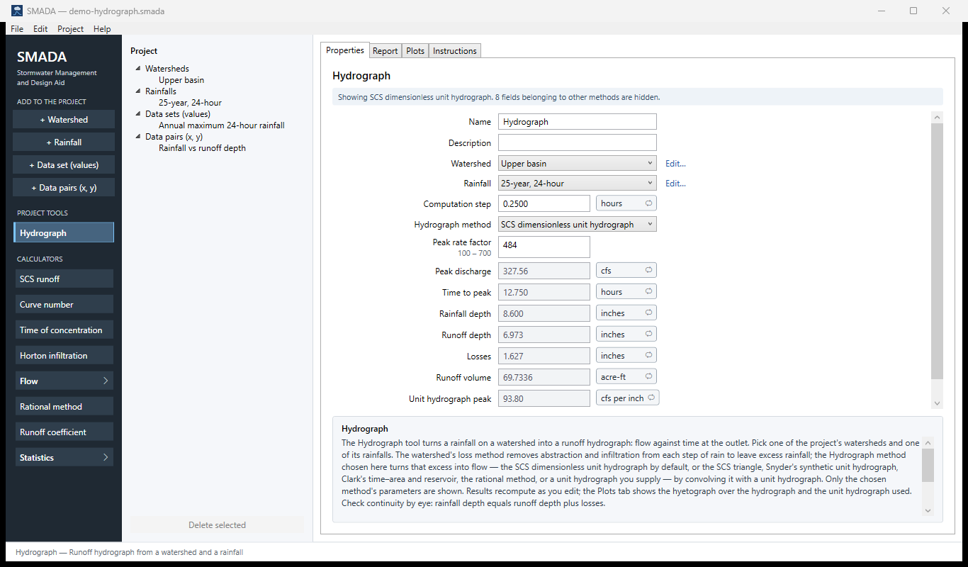
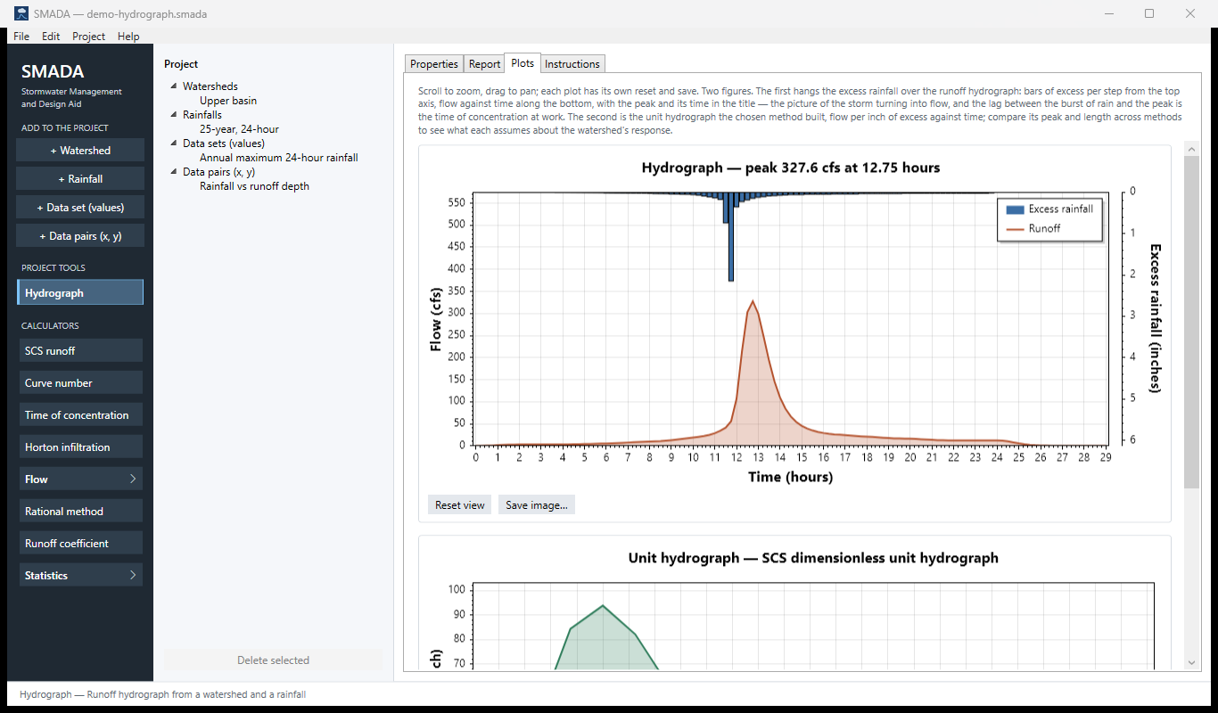
You get back the Peak discharge and its Time to peak, the Rainfall depth, Runoff depth and Losses (which always add up), the Runoff volume in acre-feet, and the peak (in cfs per inch) and timing of the unit hydrograph the method built. The Plots tab shows two plots: the first hangs the excess-rainfall bars over the runoff hydrograph, and the second shows the unit hydrograph the method built.
The pictures on this page come from the example project. In SMADA, File ▸ Open example project opens it as an untitled copy of demo-hydrograph.smada, which SMADA keeps in Documents\SMADA\Samples, so you can change anything and the example stays as it is. Its watershed, Upper basin, is 120 acres with 40 acres impervious, 30 of them directly connected, a time of concentration of 1.4 hours, and the Curve number loss method at CN 82. Its rainfall is the 25-year, 24-hour storm: 8.6 in typed at a 0.25 h step in the SCS Type II pattern from SMADA's older table. The tool is run at a 0.25 h step with the SCS dimensionless unit hydrograph and a peak rate factor of 484. If you make the storm yourself with + Rainfall, choosing Dimensionless curve, SCS Type II, 24 hour (now the NRCS TR-20 table) and a total depth of 8.6, the runoff depth is the same and the peak moves slightly, because the TR-20 storm's burst is shaped a little differently.
The Hydrograph tool is the end of SMADA's chain. The Watershed holds the land and its losses, the Time of concentration and Curve number calculators feed it, and a Rainfall supplies the storm, typed or generated from a dimensionless curve. When you need only a peak for a small paved area, the Rational method calculator is quicker.
The Hydrograph tabs
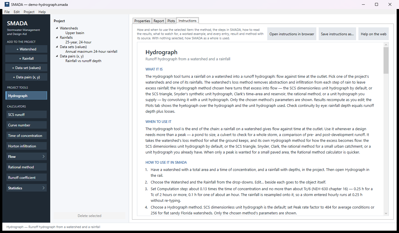
Every item in SMADA has the same four tabs. These are captured from the program with the example values it opens with (and the demo project's watershed and rainfall); select a picture to see it full size.
Download the example project (demo-hydrograph.smada: the watershed Upper basin, the 25-year, 24-hour rainfall and two data sets) and open it in SMADA with File ▸ Open to see these same numbers.
Properties tab — where you enter values and read the results
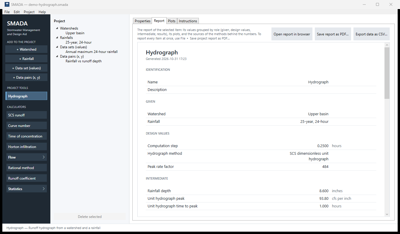
Report tab — the same values as a report, ready for HTML, PDF or CSV
Plots tab — what it draws
Instructions tab — the manual page in the program
How it calculates
Every method follows the same four steps: put the rainfall on the computation step, take the losses out to leave excess rainfall, build a unit hydrograph at the computation step, and convolve the two. The methods differ only in how the unit hydrograph is built, and the rational method also in how the excess is found. Everything is computed in base units: depths in inches, times in hours, areas in acres, flows in cfs.
Checks before anything is computed
The tool stops and shows a note above the form instead of results when:
- no watershed or no rainfall is chosen. If the project has none, the drop-down's only entry says so ("(none yet: use + Watershed)", "(none yet: use + Rainfall)") and the note says how to add one; every result shows a dash rather than a zero;
- the rainfall has no depths;
- the watershed has no total area or no time of concentration (both must be greater than zero, under every method);
- the computation step is zero or less;
- the watershed itself reports a problem: its areas disagree (directly connected impervious area larger than the impervious area, or either larger than the total), or under Horton k is not greater than 0 or fo is below fc. The note names the watershed and repeats its problem;
- the watershed has no loss method that applies (not checked under the rational method, which does not use one);
- the unit hydrograph has fewer than two ordinates (for a user-supplied unit hydrograph: enter at least two), or a unit hydrograph routine rejects its inputs (for example a time to peak of zero, or a peak rate factor the gamma shape cannot represent). The routine's own message is shown.
Step 1: the rainfall on the computation step
If the rainfall's own time step equals the computation step Δt (to within 10−9), its depths are used exactly as entered. Otherwise the storm is resampled through its dimensionless mass curve, by the same generator a Rainfall uses to build a storm from a published curve, so the total depth and the duration are kept whatever the step. The mass curve has the points (0, 0) and, after each entered depth,
F(ti) = (P1 + P2 + … + Pi) / Ptotal, ti = i Δtr
and the new increments are read from it by linear interpolation:
n = the smallest whole number with n Δt ≥ Td
P′k = Ptotal [F(min(k Δt, Td)) − F((k − 1) Δt)], k = 1 … n
with the last step closed at exactly Ptotal. When Td is not a whole number of computation steps, the last step is a partial one ending at Td, so no rain is lost.
- Pi
- entered rainfall depth in step i, in
- Ptotal
- total rainfall depth, in
- Δtr
- the rainfall's own time step, hr
- Td
- the rainfall's series duration (number of depths × Δtr), hr
- Δt
- computation step, hr
- P′k
- rainfall depth in computation step k, in
Older versions of SMADA treated each entered depth as one computation step, which compressed or stretched a storm entered at a different step; the resampling replaced that.
Step 2: excess rainfall
Under every method except the rational method, the watershed's loss method (Curve number, Horton, or Constant rate) turns each step's rainfall into excess rainfall. As in TR-55, the directly connected impervious area and the rest of the watershed each receive the whole rainfall: the connected area sheds it after its own small abstraction, the rest is reduced by the loss method, and the two runoff depths are weighted by area, Ek = fd Ed,k + fp Ep,k. The Watershed page gives the equations. Under the rational method the watershed's loss method is not used, and the excess is simply
Pe,k = C × P′k
- Pe,k
- excess rainfall in step k, in
- C
- runoff coefficient, 0 to 1 (values outside are clamped to that range)
Step 3: the unit hydrograph
A unit hydrograph is the flow at the outlet from one inch of excess spread over the watershed in one computation step. Its ordinates are in cfs per inch at times 0, Δt, 2Δt, …. The computation step is also the excess duration D of the unit hydrograph (D = Δt). Every method below ends the same way: the ordinates are scaled so the volume under them is exactly one inch (see "Scaling to one inch").
SCS dimensionless unit hydrograph (the default)
SMADA uses the gamma-function form of the NRCS curvilinear unit hydrograph. The time to peak and the peak are
Tp = D / 2 + 0.6 Tc
qp = PRF × Am / Tp, Am = A / 640
and the shape is
q(t) = qp (t / Tp)m em (1 − t / Tp)
- Tp
- time to peak from the start of the excess, hr
- D
- excess duration, equal to the computation step, hr
- Tc
- watershed time of concentration, hr (the lag is taken as 0.6 Tc)
- qp
- peak of the unit hydrograph, cfs per inch
- PRF
- peak rate factor: 484 standard, 256 for flat Florida watersheds; the form accepts 100 to 700
- A
- watershed total area, acres; Am the same in square miles
- m
- shape exponent, dimensionless
- q(t)
- unit hydrograph ordinate at time t, cfs per inch
The shape exponent m is not tabulated. SMADA solves for the m whose curve carries exactly one inch at the requested peak rate factor:
PRF(m) = 645.33 × mm+1 / [Γ(m + 1) em]
by bisection on m between 0.05 and 200, 200 halvings (Γ by the Lanczos approximation). That bracket covers peak rate factors from about 27 to 3,640; a factor outside it is refused with a note rather than clamped. A lower peak rate factor gives a smaller m: a lower peak and a longer recession for the same volume. The constant 645.33 is the flow, in cfs, of one inch over one square mile in one hour.
The curve is sampled at t = 0, Δt, 2Δt, … until it is past the peak and below 10−4 of qp; one more ordinate of exactly zero closes the recession. Because the curve is sampled, the scaled peak is close to, not exactly, PRF × Am / Tp, and the reported unit time to peak is the sample time nearest the peak.
This is a departure from the predecessor SMADA, which scaled one fixed shape: the shape exponent now follows the peak rate factor, so a 256 unit hydrograph has a longer recession, not just a lower peak.
SCS triangular unit hydrograph
The same Tp and qp as above, with straight lines up to the peak and down to the base time
Tb = 2 × 645.33 × Tp / PRF
q(t) = qp t / Tp for t ≤ Tp
q(t) = qp (Tb − t) / (Tb − Tp) for Tp < t < Tb
q(t) = 0 for t ≥ Tb
- Tb
- base time of the triangle, hr (2.67 Tp when PRF = 484)
Writing the base this way keeps the triangle's volume at one inch for any peak rate factor, not only 484.
Snyder synthetic unit hydrograph
Snyder's lag comes from two lengths, entered in feet and converted to miles:
tp = Ct (L × Lc)0.3
It is adjusted from Snyder's standard excess duration tp/5.5 to the computation step D:
tpR = tp + 0.25 (D − tp / 5.5)
Tp = max(tpR + D / 2, D)
- tp
- Snyder's standard lag, hr
- Ct
- lag coefficient, 0.1 to 10 (about 1.8 to 2.2 in Snyder's Appalachian basins)
- L
- main channel length, outlet to divide, mi (entered in ft, divided by 5280)
- Lc
- length along the channel from the outlet to the point nearest the centroid, mi
- tpR
- lag adjusted to the computation step, hr
- Tp
- time to peak from the start of the excess, hr
Snyder's peak, measured against the lag, is
qp = 640 Cp Am / tpR
The shape is the gamma unit hydrograph above, built with its peak at Tp from the start of the excess. Since the gamma form peaks at PRF × Am / Tp, SMADA gives it the peak rate factor
PRF = 640 Cp Tp / tpR
so the curve peaks at exactly Snyder's qp; the sampled ordinates match it to within the computation step.
- Cp
- Snyder's peaking coefficient, dimensionless, 0.1 to 1 (0.4 to 0.8 in most regions)
- qp
- unit hydrograph peak, cfs per inch
- PRF
- peak rate factor handed to the gamma shape, dimensionless
Before 2026-10-15 the factor was 640 Cp, which gave Snyder's peak only when D = 0. Snyder measures from the lag and the SCS form from the start of the excess, so Cp 0.75 matches the SCS 484 only roughly. Snyder gives only the peak and widths, so like HEC-HMS SMADA fits a shape to them. Every Cp from 0.1 to 1 falls inside the shape-exponent search (peak rate factors of about 27 to 3,640).
Clark unit hydrograph
The inch of excess is first translated to the outlet along the synthetic time–area curve HEC-HMS uses, over the time of concentration:
x = t / Tc
Ac(x) = 1.414 x1.5 for x ≤ 0.5
Ac(x) = 1 − 1.414 (1 − x)1.5 for 0.5 < x < 1
Ac(x) = 1 for x ≥ 1
Ii = [Ac(iΔt / Tc) − Ac((i − 1)Δt / Tc)] × Am × 645.33 / Δt
for i = 1 … ceil(Tc / Δt).
then routed through a linear reservoir:
Ca = Δt / (R + 0.5 Δt), Cb = 1 − Ca
Oi = Ca Ii + Cb Oi−1
q(iΔt) = (Oi−1 + Oi) / 2
- Ac
- cumulative fraction of the area contributing, dimensionless
- Ii
- translated inflow in step i, cfs per inch
- R
- Clark storage coefficient, hr (R = 0 sets Ca = 1: pure translation)
- Oi
- reservoir outflow at the end of step i, cfs per inch
- q
- unit hydrograph ordinate, the average of successive outflows, cfs per inch
The routing runs until the inflow has ended and the ordinate is below 10−4 of the largest so far; a final zero closes it. A larger R gives a lower, later peak with the same volume.
Rational method
The unit hydrograph is a triangle peaking at Tc with base 2 Tc (HydroCAD's form):
qp = 645.33 Am / Tc
q(t) = qp t / Tc for t ≤ Tc
q(t) = qp (2Tc − t) / Tc for Tc < t < 2Tc
q(t) = 0 for t ≥ 2Tc
With the excess C × P′k from step 2, a steady intensity i lasting at least Tc builds up to 1.008 C i A cfs (A in acres), the rational formula with its exact units constant 645.33/640. The Rational method calculator uses the same factor (43,560/12/3,600 = 1.008), so the two agree.
User-supplied unit hydrograph (S-curve)
You enter ordinates U at your own step Du, starting at time 0. They are interpolated linearly between points (and taken as zero at t ≤ 0 and at or after the last point), then converted to the computation step D′ = Δt by the S-curve method:
S(t) = Σk = 0, 1, 2 …; kDu ≤ t U(t − k Du)
U′(t) = max{ [S(t) − S(t − D′)] × Du / D′, 0 }
- U(t)
- entered unit hydrograph, flow per inch at its own step
- Du
- unit hydrograph step (its excess duration), hr
- S(t)
- S-curve: the response to excess continuing indefinitely
- D′
- new duration, the computation step, hr
- U′(t)
- converted unit hydrograph at t = 0, D′, 2D′, … up to the last entered time plus max(Du, D′)
Because the result is then scaled to one inch over the watershed, your ordinates need only be in the right proportion.
Scaling to one inch
The volume under each unit hydrograph is measured by the trapezoidal rule and converted to inches over the watershed (1 cfs for 1 hour is 3600 ft³; 1 acre-inch is 3630 ft³):
V = [Σj (qj−1 + qj) / 2 × Δt] × 3600 / 3630 / A
qj ← qj / V
- V
- volume under the sampled unit hydrograph, in over the watershed
- qj
- unit hydrograph ordinate j, cfs per inch
- A
- watershed total area, acres
Without this a coarse step leaves an error of a percent or so that every hydrograph built from the unit hydrograph would inherit.
Step 4: convolution
Each step's excess produces its own copy of the unit hydrograph, scaled by its depth and delayed to its own step, and the copies add:
Qn = Σk + j = n Pe,k × qj, tn = n Δt
- Qn
- runoff hydrograph ordinate at time tn from the start of the storm, cfs
- Pe,k
- excess rainfall in step k (k = 0 is the first step), in
- qj
- unit hydrograph ordinate j, cfs per inch
The hydrograph has (number of excess steps + number of unit ordinates − 1) ordinates. There is no fixed limit on its length; the VB3 ancestor's 260-step ceiling, which truncated long or finely stepped storms, is gone.
What it reports
- Peak discharge (cfs) and Time to peak (hr): the largest ordinate Qn and its time tn, so the time is on the computation-step grid.
- Rainfall depth = Σ P′k, in. It should equal the rainfall's own total.
- Runoff depth = Σ Pe,k, in over the whole watershed.
- Losses = Rainfall depth − Runoff depth, in. Continuity holds by construction.
- Runoff volume = Runoff depth / 12 × A, acre-ft (click the unit for cubic feet or cubic metres).
- Unit hydrograph peak (cfs per inch) and Unit hydrograph time to peak (hr): the largest ordinate of the scaled unit hydrograph and its time.
The report names the watershed and rainfall it ran, not their internal numbers, and lists the sources of the methods used. On the Plots tab the first figure's bars are labelled Excess rainfall and its title carries the peak and its time.
Choosing the computation step
The step is also the excess duration D of the unit hydrograph, so it sets how finely the peak is resolved. NEH Part 630, Chapter 16 uses D of about 0.133 Tc and no more than 0.25 Tp (about Tc/6): 0.25 hr suits a Tc of 2 hours or more, 0.1 hr one of about an hour. A coarser step flattens the peak. Halve the step and see whether Peak discharge moves; when it stops moving the step is fine. SMADA does not enforce these limits.
Checking the example by hand
The example project runs Upper basin (120 acres, 30 acres directly connected, CN 82, Tc = 1.4 hr) under the 8.6 in, 25-year, 24-hour storm, entered at 0.25 hr and run at Δt = 0.25 hr (so no resampling), using the SCS dimensionless unit hydrograph with PRF = 484.
- Runoff depth. fd = 30 / 120 = 0.25. S = 1000/82 − 10 = 2.195 in, and the curve number gives Q(8.6) = (8.6 − 0.439)2 / (8.6 + 1.756) = 6.431 in on the other 90 acres. Weighted by area: 0.25 × 8.6 + 0.75 × 6.431 = 6.973 in, the reported Runoff depth.
- Continuity. Losses = 8.600 − 6.973 = 1.627 in, the reported Losses; Rainfall depth equals the storm's own total, 8.600 in.
- Runoff volume. Runoff depth / 12 × A = 6.97336 / 12 × 120 = 69.7336 acre-ft, the reported value.
- Unit hydrograph peak. Am = 120 / 640 = 0.1875 sq mi and Tp = 0.25/2 + 0.6 × 1.4 = 0.965 hr, so qp = 484 × 0.1875 / 0.965 = 94.0 cfs per inch. SMADA reports 93.80 cfs per inch at 1.000 hr: the curve is sampled every 0.25 hr, so the largest sample falls at 1.000 hr, not at 0.965 hr, and the samples are then scaled to exactly one inch.
- Time to peak. The burst of the storm is the step that starts at 11.75 hr (2.374 in of rain); its copy of the unit hydrograph peaks 1.000 hr later, so the hydrograph peaks at 11.75 + 1.00 = 12.75 hr, the reported Time to peak. The peak, 327.56 cfs, is the sum over every step of its excess times the unit ordinate it contributes at 12.75 hr.
- Computation step. 0.133 × 1.4 = 0.19 hr and Tp/4 = 0.24 hr, so 0.25 hr is at the coarse end of NEH-630's range; run it at 0.1 hr to see how much the peak moves.
The runoff depth is worked out in more detail on the Watershed page.
Sources
- USDA NRCS, National Engineering Handbook, Part 630 Hydrology, Chapter 16 (Hydrographs), 2007.
- USDA NRCS, National Engineering Handbook, Part 630 Hydrology, Chapter 10, 2004 (SCS curve number losses).
- USDA SCS, Technical Release 55, Urban Hydrology for Small Watersheds, 2nd ed., 1986 (the SCS triangle, and Chapter 2's area weighting of the losses).
- Snyder, F. F., 'Synthetic unit-graphs', Trans. AGU 19, 1938.
- Clark, C. O., 'Storage and the unit hydrograph', Trans. ASCE 110, 1945.
- U.S. Army Corps of Engineers, HEC-HMS Technical Reference Manual, 'Snyder unit hydrograph model' and 'Clark unit hydrograph model'.
- Kuichling, E., 'The relation between the rainfall and the discharge of sewers in populous districts', Trans. ASCE 20, 1889.
- HydroCAD, 'Rational method hydrographs'.
- ASCE/WEF, Design and Construction of Urban Stormwater Management Systems, Manual 77, 1992.
- Sherman, L. K., 'Streamflow from rainfall by the unit-graph method', Engineering News-Record 108, 1932.
- Horton, R. E., Soil Science Society of America Proceedings 5, 1940 (Horton losses).
- Wanielista, Kersten and Eaglin, Hydrology: Water Quantity and Quality Control, 2nd ed., Wiley, 1997 (the SCS unit hydrograph, the S-curve and constant-rate losses).
All SMADA calculators · Get SMADA free for Windows from the Microsoft Store