Probability and distributions
Four analyses for Modules 3 to 6. None of them needs a data table: you type the probabilities or the distribution's parameters.
Probability rules (Module 3)
Two events A and B, and the probabilities that connect them: complements, the addition and multiplication rules, conditional probability, independence and Bayes' theorem — plus counting (permutations and combinations).
- How A and B relate: Independent; Mutually exclusive; P(A ∩ B) is known; P(A | B) is known; or P(B | A) and P(B | A′) are known — Bayes.
- Enter the probabilities your choice asks for (only those are shown). Each is between 0 and 1.
- Read P(A′), P(B′), P(A ∩ B), P(A ∪ B), P(A | B), P(B | A) and Independence.
- For counting, enter Items to choose from (n) and Items chosen (r) and read Permutations (nPr) and Combinations (nCr).
Watch out: mutually exclusive is not independent; P(A | B) and P(B | A) are different numbers. If the numbers you enter contradict each other (a joint probability larger than either one alone), the form says so.
Example: 1 % of parts are bad; the test flags 95 % of bad parts and 5 % of good ones. With the Bayes choice, P(bad | flagged) is about 0.16 — most flagged parts are good.
Source: EGN3443 Module 3; Montgomery and Runger, Applied Statistics and Probability for Engineers, 7th ed., Chapter 2.
Discrete distribution (Module 4)
A random variable that counts. Choose the Distribution:
- Binomial — successes in n trials: Trials (n), Success probability (p).
- Poisson — events at a mean rate: Mean rate (λ).
- Geometric — trials to the first success: p.
- Negative binomial — trials to the r-th success: Successes wanted (r), p.
- Hypergeometric — draws without replacement: Population size (N), Successes in the population (K), Draws (n).
- Typed table of (x, P(x)) — any other distribution, typed as pairs.
Enter the Value of interest (k) and, for a range, an Upper value (k₂). Read P(X = k), P(X ≤ k), P(X < k), P(X ≥ k), P(X > k), P(k ≤ X ≤ k₂), the mean, variance and standard deviation. Plots shows the bars of P(X = x) with your values shaded, and the cumulative staircase.
Watch out: "at least k" is P(X ≥ k), "more than k" is P(X ≥ k + 1). The geometric and negative binomial count trials (including the success), as the course does. The Poisson rate must match the interval: 3 per hour is λ = 6 for two hours.
Example: ten items from a line that is 10 % defective (binomial, n = 10, p = 0.1): P(X = 0) = 0.349, P(X ≤ 2) = 0.930, P(X ≥ 3) = 0.070.
Source: EGN3443 Module 4; Montgomery and Runger, Applied Statistics and Probability for Engineers, 7th ed., Chapter 3.
Continuous distribution (Module 5)
A random variable that measures — and the table look-ups of the course. Choose the Distribution: Uniform (a, b), Normal (μ, σ), Exponential (rate λ), Lognormal (μ and σ of ln X), Student's t (ν), Chi-squared (ν) or F (ν₁, ν₂).
- Enter the parameters, the Value of interest (x) and optionally an Upper value (x₂).
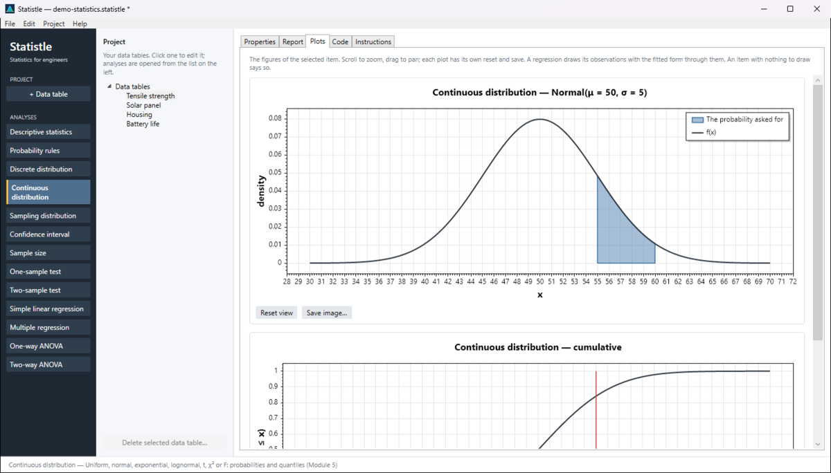
- Read the Density f(x), P(X ≤ x), P(X > x), P(x ≤ X ≤ x₂), and for the normal the z-score of x.
- For the reverse question — which x has P(X ≤ x) = q — enter the Probability for the quantile (q) and read Quantile x with P(X ≤ x) = q.
Reading it: for a continuous variable, probabilities are areas; the density is a height, not a probability. Plots shades the area.
Watch out: the exponential uses the rate λ (mean 1/λ); Python's scipy uses scale = 1/λ, and the generated code says so. The lognormal's μ and σ describe ln X, not X.
Example: shaft diameters normal with μ = 25.00 mm, σ = 0.02 mm: P(X ≤ 24.97) = 0.067 (z = −1.5); the diameter exceeded by 5 % of shafts (q = 0.95) is 25.033 mm.
Source: EGN3443 Module 5; Montgomery and Runger, Applied Statistics and Probability for Engineers, 7th ed., Chapter 4.
Sampling distribution (Module 6)
What a sample mean or proportion does over repeated samples. Choose the Statistic (Sample mean x̄ or Sample proportion p̂), enter the population mean μ and standard deviation σ (or the proportion p), the Sample size (n), and the value of interest (and an optional upper value).
Read the mean of the sampling distribution, the Standard error, the z for the value, P(statistic ≤ value), P(statistic ≥ value), the range probability, the middle 95 %, and whether the normal approximation is adequate. Plots draws the population beside the much narrower sampling distribution of the mean.
Watch out: σ/√n is the spread of the mean, not of the data. A skewed population needs n around 30 for the central limit theorem. This analysis assumes σ is known; when you only have s from a sample, use the t-based analyses.
Example: bolts with μ = 4200 N, σ = 350 N. For n = 5 the standard error is 156.5 N and P(x̄ ≤ 4000) = 0.10; for n = 30 it is 63.9 N and the probability falls to 0.001.
Source: EGN3443 Module 6; Montgomery and Runger, Applied Statistics and Probability for Engineers, 7th ed., Chapter 7.
The help panel, Report and Instructions tabs name the source of each method in use, and the Code tab writes each calculation in Python (scipy.stats) and R.
← Descriptive statistics Confidence intervals and sample size →