Hypothesis tests
Use a test when the question contains a claim — "the mean is 50", "no more than 5 % defective", "the new supplier is no different". Both analyses report the hypotheses, the test statistic, the rejection region, the p-value, the Decision in words and the confidence interval that goes with the test.
One-sample test (Modules 8–9)
- Test: Mean, σ known (z-test); Mean, σ unknown (t-test); Proportion (z-test); or Variance (χ²-test).
- Alternative hypothesis: Two-sided (≠), Less than (<) or Greater than (>) — chosen from the wording of the question, before looking at the data.
- Significance level (α), usually 0.05, and the Null value (μ₀, p₀ or σ₀).
- Data from: summary statistics you type, or a column of a data table.
- Optional: a True mean worth detecting (μ₁) and a Target power, to read Power at μ₁ and the n for the target power.
Reading it: reject H₀ when the statistic falls in the rejection region — the same as p < α. The p-value is the chance of a result at least this extreme if H₀ were true; it is not the chance that H₀ is true. Not rejecting is not proof of H₀ — check the power.
Watch out: the t-test assumes a roughly normal population when n is small. The proportion z-test needs np₀ and n(1 − p₀) both large enough (the help says how large). The variance test is sensitive to non-normal data.
Example: 25 specimens, mean 51.3, against μ₀ = 50 with σ = 2, greater than, α = 0.05: z = 3.25, p = 0.0006, reject (Montgomery and Runger, Example 9-2). Plots shows the reference distribution with the rejection region shaded and your statistic marked.
Two-sample test (Modules 9–10)
- Test, by the design: Two means, equal variances (pooled t); Two means, unequal variances (Welch t); Paired samples (paired t); Two means, σ₁ and σ₂ known (z); Two proportions (pooled z); Two variances (F); Mann–Whitney U (non-parametric, independent); Wilcoxon signed-rank (non-parametric, paired).
- Alternative hypothesis and Significance level (α).
- Hypothesised difference (Δ₀) — 0 unless the claim names a difference.
- Data from: summaries for each sample, or two columns of a data table. With columns, Statistle also reports Effect size (Cohen's d), Shapiro–Wilk normality checks on each sample and Levene's equal-variance check. The rank tests (Mann–Whitney, Wilcoxon) need the data itself, so they need columns.
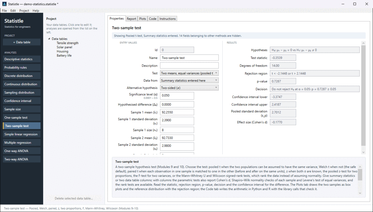
Reading it: a small p says the groups differ; the confidence interval on the difference says by how much, in your data's units — usually what matters more. Cohen's d: 0.2 small, 0.5 medium, 0.8 large. Levene p below 0.05 argues for Welch over pooled; Shapiro–Wilk p below 0.05 in a small sample argues for the rank tests.
Watch out: when in doubt, use Welch. A paired test needs the two columns the same length and in matching order — and analysing paired data as independent throws away the pairing's advantage. Mann–Whitney compares distributions, not means.
Example: in the sample project, pick two alloy columns of Tensile strength as the two samples to see the checks and the side-by-side box plots appear.
Where the formulas come from
EGN3443 Modules 8–10; Montgomery and Runger, Applied Statistics and Probability for Engineers, 7th ed., Chapters 9 and 10. The Instructions tab and the Report tab name the source of every method in use, and the help panel shows it when you click a field. The Code tab writes the same calculation in Python and R, formula first.