Regression
Simple linear regression (Modules 11 and 13)
One response y that depends on one predictor x: how much y changes per unit of x, whether there is a relation at all, and a prediction at a new x with an honest interval.
- Choose the x column (the predictor) and the y column (the response), or choose Entered below and type the pairs into Data (x, y), one pair per line (or use its Import…).
- Leave Transform x and Transform y at None for a straight line. If the residual plot curves, try Natural log (ln), Square root (√) or Reciprocal (1/) and compare.
- Enter the Confidence level, and optionally Predict at x₀.
- Read the Equation, Intercept (b₀) and Slope (b₁) with standard errors, the slope's t, p-value and confidence interval, Correlation (r), R², the Residual standard error (σ̂) and the ANOVA F.
- With x₀: the Fitted y at x₀ with the interval for the mean response and the wider interval for one new observation.
- Diagnostics: Durbin–Watson, Shapiro–Wilk of the residuals, the largest Cook's distance and leverage, and the most influential observation.
Reading it: the slope answers most engineering questions — its interval says how well it is known, its p-value whether it could be zero. R² is the share of y's variation the line explains; σ̂ is the typical miss in y's units. Durbin–Watson near 2, Shapiro–Wilk p above 0.05 and Cook's distances well below 1 say the assumptions hold.
Watch out: do not predict outside the range of x. A high R² does not make the model right; a curved residual plot makes it wrong. A log transform cannot take zero or negative values — the form counts the pairs it skipped. One influential point can steer the whole line.
Plots: the data with the fitted line (or curve), residuals against fitted values, and the normal Q–Q plot of the residuals.
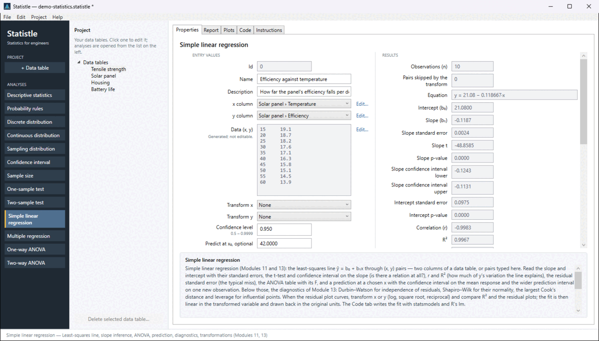
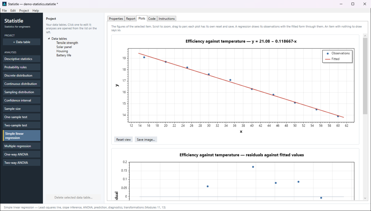
Example: the sample project's Solar panel analysis — efficiency against cell temperature, ten pairs, slope about −0.119 % per °C, R² above 0.99.
Multiple regression (Modules 12–13)
A response that depends on several predictors at once: each predictor's effect with the others held fixed, which predictors earn their place, which overlap, and how well the model predicts new data.
- Put the response and predictors in one data table, one column each, all the same length. Choose the Data table and the Response column (y).
- Predictor columns: type their names separated by commas, or leave blank to use every other column.
- Variable selection: All the predictors listed first; then try Forward selection (add while p < 0.05) or Backward elimination (drop while p ≥ 0.05) and compare.
- Confidence level, and Cross-validation folds (k) — 5 or 10; 0 to skip.
- Read the Coefficients table (estimate, standard error, t, p, interval and VIF per term), R² and Adjusted R², σ̂, the F-test, the diagnostics, and the In-sample RMSE against the Cross-validated RMSE.
Reading it: compare models by adjusted R² (plain R² only ever rises as terms are added). A VIF above 5 to 10 means that predictor overlaps the others and its coefficient cannot be trusted alone. A cross-validated RMSE far above the in-sample RMSE means overfitting.
Watch out: selection is exploratory — say you used it, and prefer the model that makes engineering sense. Collinear predictors make the fit impossible; the form says so — drop one. You need comfortably more rows than predictors.
Plots: observed against predicted, residuals against fitted, and the Q–Q plot.
Example: the sample project's Housing table — price on size, age, bedrooms and distance for twenty houses. Try backward elimination and see which predictors survive.
Where the formulas come from
EGN3443 Modules 11–13; Montgomery and Runger, Applied Statistics and Probability for Engineers, 7th ed., Chapters 11 and 12. The Instructions tab and the Report tab name the source of every method in use, and the help panel shows it when you click a field. The Code tab writes the same calculation in Python and R, formula first.